1 Concepts and terminology
This chapter briefly introduces the concepts and terminology of SECR. The following chapter gives a simple example. Technical details are provided in the Theory chapters.
1.1 Motivation
“Measurement of the size of animal populations is a full-time job and should be treated as a worthy end in itself.”
S. Charles Kendeigh (1944)
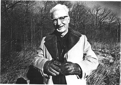
Photo: L.L.Getz
Only a brave ecologist would make this claim today. Measuring animal populations is now justified in more practical terms - the urgent need for evidence to track biodiversity decline or to manage endangered or pest species or those we wish to harvest sustainably. But we rather like Kendeigh’s formulation, to which could be added the lure of the statistical challenges. This book has no more to say about the diverse reasons for measuring populations: we will focus instead on a particular toolkit.
Populations of some animal species can be censused by direct observation, but many species are elusive or cryptic. Surveying these species requires indirect methods, often using passive devices such as traps or cameras that accumulate records over time. Passive devices encounter animals as they move around. The scale of that movement is unknown, which creates uncertainty regarding the population that is sampled. Furthermore, the number of observed individuals increases indefinitely as more and more peripheral individuals are encountered1.
SECR cuts through this problem by modelling the spatial scale of detection to obtain an unbiased estimate of the stationary density of individuals.
1.2 State and observation models
It helps to think of SECR in two parts: the state model and the observation model (Borchers et al., 2002). The state model describes the biological reality we wish to describe, the animal population. The observation model represents the sampling process by which we learn about the population. The observation model matters only as the lens through which we can achieve a clear view of the population. We treat the state model (spatial population) and observation model (detection process) independently, with rare exceptions (Section 5.10).
1.3 Spatial population
An animal population in SECR is a spatial point pattern. Each point represents the location of an animal’s activity centre, often abbreviated AC.
Statistically, we think of a particular point pattern, a particular distribution of AC, as just one possible outcome of a random process. Run the process again and AC will land in different places and even differ in number. We equate the intensity of the random process with the ecological parameter ‘population density’. This formulation is more challenging than the usual “density = number divided by area”, but it opens the door to rigorous statistical treatment.
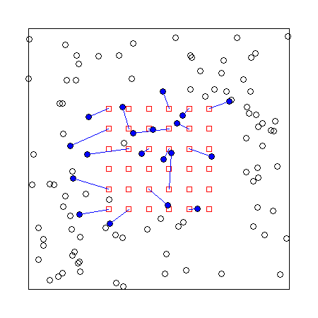
The usual process model is a 2-dimensional Poisson process (Fig. 1.1). By fitting the SECR model we can estimate the intensity surface of the Poisson process that we represent by D(\mathbf x) where \mathbf x stands for the x,y coordinates of a point. Density may be homogeneous (a flat surface, with constant D(\mathbf x)) or inhomogeneous (spatially varying intensity). Inhomogeneous density may differ discretely, between habitats, or continuously in response to mapped covariates.
An inhomogeneous intensity surface is considered to depend on a vector of parameters \phi, hence D(\mathbf x; \phi). For constant density \phi is a single value. If there are two habitats \phi provides a value for each one. If density varies linearly with a covariate then \phi comprises the intercept and slope.
Activity centre vs home range centre
‘Activity centre’ is often used in preference to ‘home range centre’ because it appears more neutral. ‘Home range’ implies a particular pattern of behaviour: spatial familiarity and repeated use in contrast to nomadism. However, SECR assumes the very pattern of behaviour (persistent use) that distinguishes a home range, and it is safe to use ‘activity centre’ and ‘home range centre’ interchangeably in this context.
1.4 Detectors
Basic SECR uses sampling devices (‘detectors’) placed at known locations. We need to recognise individuals whenever they are detected. At least some of the individuals should be detected at multiple locations. The accumulated detections of each known individual are its ‘detection history’. Device types differ according to how they affect animal behaviour and the data they collect (Table 1.1). The term ‘detector type’ groups devices according to the required probability model (Section 3.4).
Detection may be entirely passive and non-invasive if individuals carry unique natural marks (e.g., pelage patterns) or their DNA can be sampled. Devices that record detections passively are “proximity detectors”. Proximity detectors may be split according to the distribution of the number of detections per animal per occasion (binary, Poisson, or binomial), with binary being the most common2.
Animals without natural marks must be marked individually on their first detection. This implies capture and handling. Only devices that hold an animal until it is released can truly be called ‘traps’.3 The probability model for trapping must allow for exclusivity: an animal can be found at only one trap on any occasion, and some traps (‘single-catch’ traps) also exclude other individuals after the first.
| Device | Marks | Detector type | Example |
|---|---|---|---|
| Automatic camera | natural marks: stripes and spots | proximity | tiger, Royle et al. (2009) |
| Hair snag | microsatellite DNA | proximity | grizzly bear, Mowat & Strobeck (2000) |
| Cage trap | numbered ear tag | single-catch trap | brushtail possum, Efford et al. (2005) |
| Ugglan trap | numbered ear tag | multi-catch trap | field vole, Ergon & Gardner (2013) |
| Mist net | numbered leg band | multi-catch trap | red-eyed vireo, Borchers & Efford (2008) |
1.5 Area search
The preceding description assumes sampling at discrete points in space. Searches may also be conducted across space, yielding a possibly unique location for each detection. There are parallel SECR models for such data (Chapter 4, Appendix D). Searched areas are somewhat analogous to detectors, and may or may not allow only one detection per occasion, like true traps. Data from area searches may be easier to analyse if they are discretized and treated as coming from many point detectors.
1.6 Sampling across time
For most vertebrates we expect population turnover (births, deaths, AC movement) on a time scale of months or years. Population change is often negligible over shorter spans (days or weeks, depending on the species, time of year etc.). Sampling over shorter spans can therefore treat the size and composition of a population as fixed: it is said to be ‘closed’. This greatly simplifies analysis. We assume closure except when considering breaches of assumptions.
A set of samples from a closed population comprises a sampling ‘session’. For trap-type detectors there must be multiple ‘occasions’ within a sampling session to obtain recaptures. For proximity-type detectors the role of occasions is more subtle, and data may usually be collapsed to animal- and detector-specific counts. The spatial pattern of binary detections alone is sufficient to obtain an estimate of density (Efford et al., 2009).
Continuous time
Some devices such as automatic cameras record data in continuous time. Detection events are stamped with the clock time and date, rather than assigned to discrete occasions. SECR models may be written for continuous time data, and these models have mathematical elegance. They find practical application in some niche cases (e.g. Distiller & Borchers, 2015).
It is not necessary for all detectors to be used on all occasions. Incomplete usage (and other variation in effort per occasion – Efford et al., 2013) may be recorded for each detector and allowed for in the analysis.
Data collected across multiple sessions potentially include the loss of some individuals and recruitment of others. An open population model is the natural way to go (e.g., Efford & Schofield, 2020). However, the complexity of open-population models can be avoided if sessions are treated as independent in a ‘multi-session’ closed population analysis (Chapter 14).
1.7 Data structure
Data for a single SECR session comprise a 3-dimensional rectangular array with dimensions corresponding to known animals, sampling occasions, and detectors. Data in each cell of the array are usually binary (0/1) but may be integer counts > 1 (e.g., if binary data have been collapsed by occasion). In secr, an R object of class ‘capthist’ holds data in this form, along with the coordinates of the detectors in its ‘traps’ attribute. The user constructs a capthist object from text or spreadsheet input using data entry functions described in Chapter 9.
1.8 Model fitting
A SECR model combines a model for the point process (the state model) and a model for distance-dependent detection (the observation model). Unbiased estimates of population density (and other parameters) are obtained by jointly fitting the state and observation models.
1.8.1 Distance-dependent detection
In order to estimate density from a sample we must account for the sampling process. The process is inherently spatial: each animal is more likely to be detected near its AC, and less likely to be detected far away. Sampling filters the geographic locations of animals as indicated in Fig. 1.1.
The true locations of animals are not known, and therefore the distance-dependent probabilities cannot be calculated directly. The model is fitted by marginalising (integrating over) animal locations.
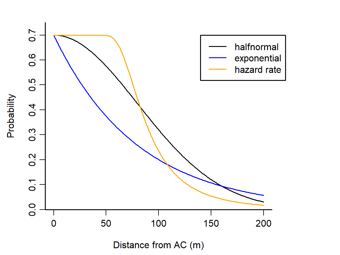
Distance-dependent detection is represented by a ‘detection function’ with intercept, scale, and possibly shape, determined by parameters to be estimated4.
1.8.2 Habitat
SECR models include a map of potential habitat near the detectors. Here ‘potential’ means ‘feasible locations for the AC of detected animals’. Excluded are sites that are known a priori to be unoccupied, and sites that are so distant that an animal centred there has negligible chance of detection.
The habitat map is called a ‘habitat mask’ in secr and a ‘state space’ in the various Bayesian implementations. It is commonly formed by adding a constant-width buffer around the detectors. For computational convenience the map is discretized as many small pixels. Spatial covariates (vegetation type, elevation, etc.) may be attached to each pixel for use in density models. Buffer width and pixel size are considered in Chapter 12. The scale at which spatial covariates affect density is considered separately.
1.8.3 Link functions
A simple SECR model has three parameters: density D, and the intercept g_0 and spatial scale \sigma of the detection function. Valid values of each parameter are restricted to part of the real number line (positive values for D and \sigma, values between zero and one for g_0). A straightforward way to constrain estimates to valid values is to conduct maximization of the likelihood on a transformed (‘link’) scale: at each evaluation the parameter value is back transformed to the natural scale. The link function for all commonly used parameters defaults to ‘log’ (for positive values) except for g0 which defaults to ‘logit’ (for values between zero and one).
| Name | Function | Inverse |
|---|---|---|
| log | y = \log(x) | \exp(y) |
| logit | y = \log[p/(1-p)] | 1 / [1 + \exp(-y)] |
| identity | y=x | y |
| cloglog | y = \log(-\log(1-p)) | 1 -\exp(-\exp(y)) |
Working on a link scale is especially useful when the parameter is itself a function of covariates. For example, \log (D) = \beta_0 + \beta_1 c \; for a log-linear function of a spatially varying covariate c. The coefficients \beta_0 and \beta_1 are estimated in place of D per se.
We sometimes follow MARK (e.g., Cooch & White, 2023) and use ‘beta parameters’ for coefficients on the link scale and ‘real parameters’ for the core parameters (D, g_0, \lambda_0, \sigma) on the natural scale.
1.8.4 Estimation
There are several ways to estimate the parameters of the SECR probability model, all of them computer-intensive. We focus on numerical maximization of the log likelihood (Borchers & Efford (2008) and Chapter 3). The likelihood integrates over the unknown locations of the animals’ activity centres. This is achieved in practice by summing over cells in a discretized map of the habitat.
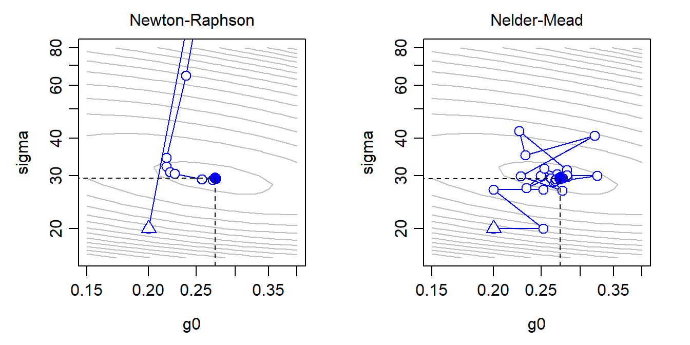
In outline, a function to compute the log likelihood from a vector of beta parameters is passed, along with the data, to an optimization function. Optimization is iterative. For illustration, Fig. 1.3 shows the sequence of likelihood evaluations with two maximization algorithms when the parameter vector consists of only the intercept and spatial scale of detection. Optimization returns the maximized log likelihood, a vector of parameter values at the maximum, and the Hessian matrix from which the variance-covariance matrix of the estimates may be obtained.
Bayesian methods make use of algorithms that sample from a Markov chain (MCMC) to approximate the posterior distribution of the parameters. MCMC for abundance estimation faces the special problem that an unknown number of individuals, at unknown locations, remain undetected. The issue is addressed by data augmentation (Royle & Young, 2008) or using a semi-complete data likelihood (King et al., 2016).
Early anxiety about the suitability of MLE and asymptotic variances for SECR with small samples appears to have been mistaken. Royle et al. (2009) believed that “… the practical validity of these procedures cannot be asserted in most situations involving small samples”. This has not been borne out by subsequent simulations. The final discussion of Gerber & Parmenter (2015) is pertinent: they give an even-handed summary of the philosophical and practical issues, and suggest that “the asymptotic argument against likelihood methods for SCR is moot.” Palmero et al. (2023) reported that Bayesian methods provide more precise estimates of density, but this appears to be an artefact: it is a mistake to compare estimates from MLE models with random N(A) with estimates from Bayesian models with fixed N(A) (see Section 3.5 for background on N(A), the population in area A).
The choice between Bayesian and frequentist (MLE) methods is now an issue of convenience for most users:
- MLE provides fast and repeatable results for established models with a small to medium number of parameters.
- Bayesian methods have an advantage for novel models and possibly for those with many parameters.
Bayesian priors are usually chosen to be ‘uninformative’, and under these conditions the mode of the posterior distribution is expected to be a close match to the maximum likelihood estimate. Informative priors, perhaps based on estimates of detection parameters from past studies, are a way to make something out of very sparse datasets. Their use must be fully reported and explained.
A further method, simulation and inverse prediction, has a niche use for data from single-catch traps (Efford et al., 2004; Efford, 2023).
For a bounded population the number of observed individuals has a natural limit, the true population size. Even when it exists, this is not usually the number that would be estimated by non-spatial capture–recapture (Otis et al., 1978).↩︎
In the secr software, type ‘proximity’ refers specifically to binary proximity detectors.↩︎
Confusingly, secr uses ‘traps’ as a generic name for R objects holding detector coordinates and other information. This software-specific jargon should be avoided in publications.↩︎
All detection functions have intercept (g_0, \lambda_0) and scale (\sigma) parameters; some such as the hazard rate function have a further parameter that controls some aspect of shape.↩︎