Appendix F — Non-Euclidean distances

Spatially explicit capture–recapture (SECR) entails a distance-dependent observation model: the expected number of detections (\lambda) or the probability of detection (g) declines with increasing distance between a detector and the home-range centre of a focal animal. ‘Distance’ here usually, and by default, means the Euclidean distance. The observation model can be customised by replacing the Euclidean distance with one that ‘warps’ space in some ecologically meaningful way. There are innumerable ways to do this. One is the non-Euclidean ‘ecological distance’ envisioned by Royle et al. (2013). Redefining distance is a way to model spatial variation in the size of home ranges, and hence the spatial scale of movement \sigma; Efford et al. (2016) used this to model inverse covariation between density and home range size. Distances measured along a linear habitat network such as a river system are also non-Euclidean (see package secrlinear).

This document shows how to define and use non-Euclidean distances in secr. Code is included for the non-Euclidean SECR simulation of Sutherland et al. (2015).

F.1 Basics

The Euclidean distance between points (x_1,y_1) and (x_2,y_2) is given by d = \sqrt{(x_1-x_2)^2 + (y_1 - y_2)^2}. Non-Euclidean distances are defined in secr by setting the ‘userdist’ component of the ‘details’ argument of secr.fit. The options are (i) to provide a static (pre-computed) K \times M matrix containing the distances between the K detectors and each of the M mask points, or (ii) to provide a function that computes the distances dynamically. A static distance matrix can allow for barriers to movement. Providing a function is more flexible and allows the estimation of a parameter for the distance model, but evaluating the function for each likelihood slows down model fitting.

F.2 Static userdist

A pre-computed non-Euclidean distance matrix may incorporate constraints on movement, particularly mapped barriers to movement, and this is the most obvious reason to employ a static userdist. The function nedist builds a suitable matrix.

As an example, take the 1996 DNA survey of the grizzly bear population in the Central Selkirk mountains of British Columbia by Mowat & Strobeck (2000). Their study area was partly bounded by lakes and reservoirs that we assume are rarely crossed by bears. To treat the lakes as barriers in a SECR model we need a matrix of hair snag – mask point distances for the terrestrial (non-Euclidean) distance between each pair of points.

We start with the hair snag locations CStraps and a SpatialPolygonsDataFrame object BLKS_BC representing the large lakes (Fig. F.1). Buffering 30 km around the detectors gives a naive mask (Fig. F.1 b); we use a 2-km pixel size and reject points centred in a lake. The shortest dry path from many points on the naive mask to the nearest detector is much longer than the straight line distance.

CSmask2000 <- make.mask (CStraps, buffer = 30000, 
    type = "trapbuffer", spacing = 2000, poly = BLKS_BC, 
    poly.habitat = FALSE, keep.poly = FALSE)

par(mfrow = c(1,2), mar = c(1,4,1,4), cex = 1.6, col = "black")
plot(CStraps, gridl = FALSE, border = 30000)
selectedlakes <- c(1730, 2513, 2514, 2769, 2686, 2749)
plot(BLKS_BC[selectedlakes,], col = "blue", add = TRUE)
text(1546000, 510000, "a.", xpd = TRUE, col = "black")

plot(CStraps, gridl = FALSE, border = 30000, hidetr = TRUE)
plot(CSmask2000, dots = FALSE, add = TRUE)
plot(CStraps, add = TRUE)
par(col = "black", cex = 1.6)
text(1537000, 510000, "b.", xpd = TRUE)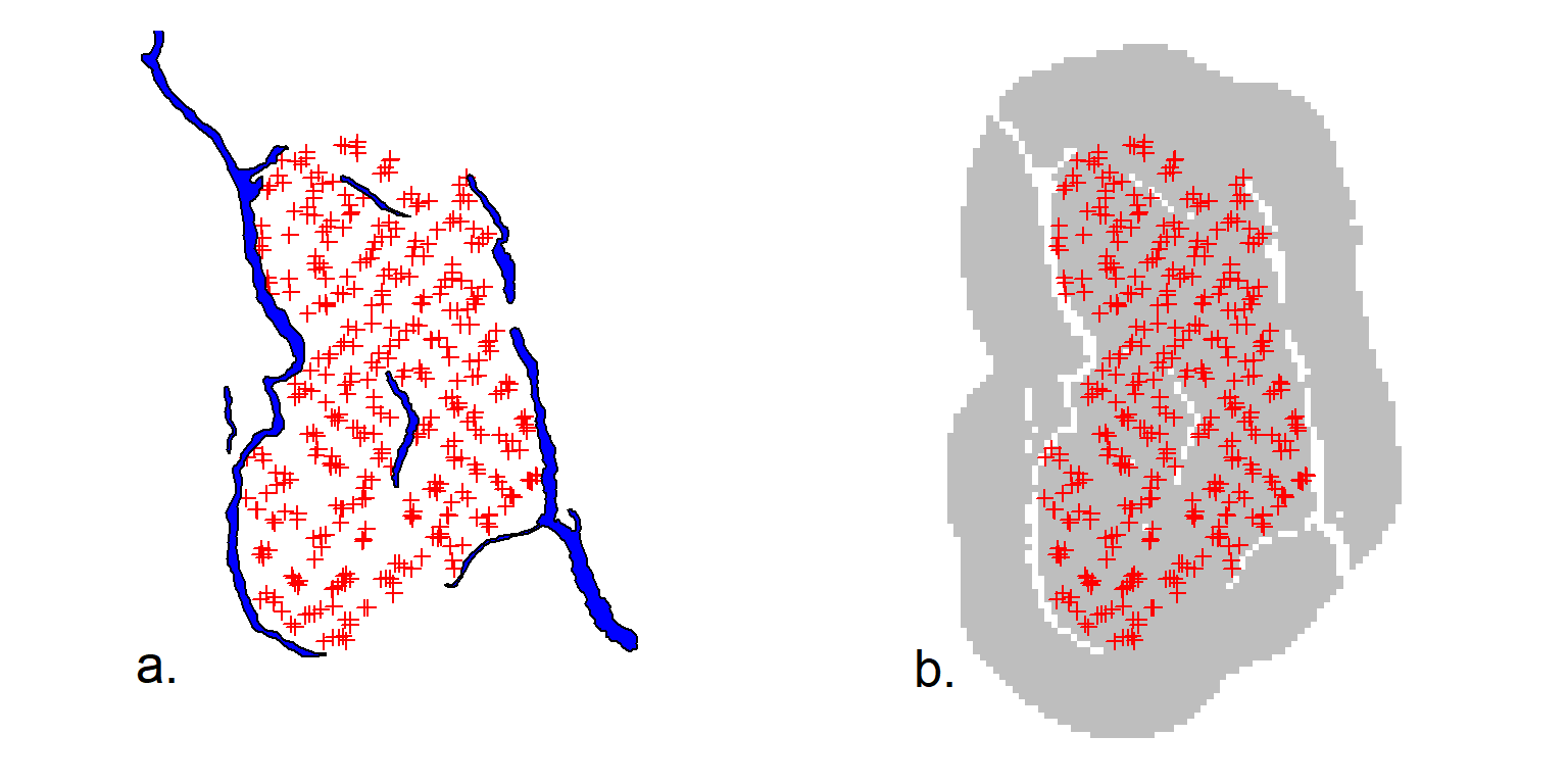

Figure F.1: (a) Central Selkirk grizzly bear hair snag locations, (b) Mask using naive 30-km buffer around hair snags.

We next calculate the matrix of all dry detector–mask distances by calling nedist that in turn uses functions from the R package gdistance (van Etten, 2023). Missing pixels in the mask represent barriers to movement when their combined width exceeds a threshold determined by the adjacency rule in gdistance.

What do we mean by an adjacency rule? gdistance finds least-cost distances through a graph formed by joining ‘adjacent’ pixels. Adjacent pixels are defined by the argument ‘directions’, which may be 4 (rook’s case), 8 (queen’s case) or 16 (knight and one-cell queen moves) as in the raster function adjacent. The default in nedist is ‘directions = 16’ because that gives the best approximation to Euclidean distances when there are no barriers. The knight’s moves are \sqrt 5 \approx 2.24 \times cell width (‘spacing’), so the width of a polygon intended to map a barrier should be at least 2.24 \times cell width.

Some of the BC lakes are narrow and less than 4.48 km wide. To ensure these act as barriers we could simply reduce the spacing of our mask, but that would slow down model fitting. The alternative is to retain the 2-km mask for model fitting and to define a finer (0.5-km) mask purely for the purpose of computing distances¹:

CSmask500 <- make.mask (CStraps, buffer = 30000, type = 
    "trapbuffer", spacing = 500, poly = BLKS_BC, poly.habitat =
     FALSE, keep.poly = FALSE)
userd <- nedist(CStraps, CSmask2000, CSmask500)

The first argument of nedist provides the rows of the distance matrix and the second argument the columns; the third (if present) defines an alternative mask on which to base the calculations. To verify the computation, map the distance from a chosen detector i to every point in a mask. Here is a short function to do that (example in Fig. F.2 a).

# map non-Euclidean distance from detector i 
# or arbitrary point on existing plot (i = NA)
dmap <- function (traps, mask, userd, i = 1, ...) {
    if (is.na(i)) i <- nearesttrap(unlist(locator(1)), traps)
    covariates(mask) <- data.frame(d = userd[i,])
    covariates(mask)$d[!is.finite(covariates(mask)$d)] <- NA  
    plot(mask, covariate = "d", ...)  
    points(traps[i,], pch = 3, col = "red")
}

At this point we could simply use ‘userd’ as our userdist matrix. However, CSmask2000 now includes a lot of points that are further than 30 km from any detector. It is better to drop these points and the associated columns of ‘userd’ (Fig. F.2 b):

OK <- apply(userd, 2, min) < 30000
CSmask2000b <- subset(CSmask2000, OK)
userdx <- userd[,OK]

par(mfrow = c(1,2), mar = c(1,4,1,4), cex = 1.1, col = "black")

dmap(CStraps, CSmask2000, userd, dots = FALSE, scale = 0.001, 
     title = "km")
par(cex = 1.6)
text(1537000, 510000, "a.", xpd=T, col="black")

plot(CStraps, gridl = FALSE, border = 30000, hidetr = TRUE)
plot(CSmask2000b, dots = FALSE, add = TRUE)
plot(CStraps, add = TRUE); par(col = "black", cex = 1.6)
text(1537000, 510000, "b.", xpd = TRUE, col = "black")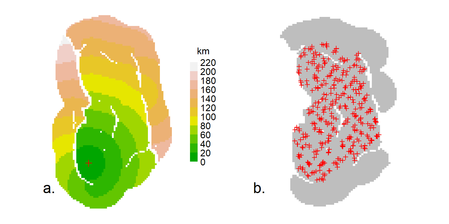

Figure F.2: (a) Central Selkirk dry-path distances from an arbitrary point (+), and (b) Efficient mask rejecting dry-path distances >30km.

Finally, we can fit a model using the non-Euclidean distance matrix:

CSa <- secr.fit(CS_sexcov_all, mask = CSmask2000b, 
    details = list(userdist = userdx))
predict(CSa)                

For completeness, note that Euclidean distances may also be pre-calculated, using the function edist. By default, secr.fit uses that function internally, and there is usually little speed improvement when the calculation is done separately.

F.3 Dynamic userdist

For dynamic non-Euclidean distances a function is passed to secr.fit in the ‘details’ argument ‘userdist’, rather than a matrix. The userdist function should take three arguments. The first two are simply 2-column matrices with the coordinates of the detectors and animal locations (mask points) respectively. The third is a habitat mask (this may be the same as xy2). The function has this form:

mydistfn <- function (xy1, xy2, mask) {
  if (missing(xy1)) return(charactervector)  
  ...
  distmat  # return nrow(xy1) x nrow(xy2) matrix
}

Computation of the distances is entirely under the control of the user – here we indicate that by ‘…’. The calculations may use cell-specific values of two ‘real’ parameters ‘D’ and ‘noneuc’ that as needed are passed by secr.fit as covariates of the mask. ‘D’ is the usual cell-specific expected density in animals per hectare. ‘noneuc’ is a special cell-specific ‘real’ parameter used only here: it means whatever the user wants it to mean.

Whether ‘noneuc’, ‘D’ or other mask covariates are needed by mydistfn is indicated by the character vector returned by mydistfn when it is called with no arguments. Thus, charactervector may be either a zero-length character vector or a vector of one or more parameter names (“noneuc”, “D”, c(“noneuc”, “D”)).

‘noneuc’ has its own link scale (default ‘log’) on which it may be modelled as a linear function of any of the predictors available for density (x, y, x2, y2, xy, session, Session, g, or any mask covariate – see Chapter 11. It may also, in principle, be modelled using regression splines (Borchers & Kidney, 2014), but this is untested. When the model is fitted by secr.fit, the beta parameters for the ‘noneuc’ sub-model are estimated along with all the others. To make noneuc available to userdist, ensure that it appears in the ‘model’ argument. Use the formula noneuc ~ 1 if noneuc is constant.

The function may compute least-cost paths via intervening mask cells using the powerful igraph package (Csardi & Nepusz, 2006). This is most easily accessed with package gdistance, which in turn uses the RasterLayer S4 object class from the package raster. To facilitate this, secr includes code to treat the ‘mask’ S3 class as a virtual S4 class, and provides a method for the function ‘raster’ to convert a mask to a RasterLayer.

If the function generates any bad distances (negative, infinite or missing) these will be replaced by 1e10, with a warning.

F.4 Examples

We use annotated examples to show how the userdist function may be used to define different models. For illustration we use the Orongorongo Valley brushtail possum dataset from February 1996 (OVpossumCH). The data are captures of possums over 5 nights in single-catch traps at 30-m spacing. We start by extracting the data, defining a habitat mask, and fitting a null model:

datadir <- system.file("extdata", package = "secr")
ovforest <- sf::st_read (paste0(datadir, "/OVforest.shp"), 
    quiet = TRUE)
ovposs <- OVpossumCH[[1]]  # select February 1996
ovmask <- make.mask(traps(ovposs), buffer = 120, type = "trapbuffer", 
    poly = ovforest[1:2,], spacing = 7.5, keep.poly = FALSE)
# for plotting only
leftbank <- read.table(paste0(datadir,"/leftbank.txt"))[21:195,]

fit0 <- secr.fit(ovposs, mask = ovmask, detectfn = "HHN", trace = FALSE)

Warning: multi-catch likelihood used for single-catch traps

The warning is routine: we will suppress it in later examples. The distance functions below are not specific to a particular study: each may be applied to other datasets.

F.4.1 Scale of movement \sigma depends on location of home-range centre

In this simple case we use the non-Euclidean distance function to model continuous spatial variation in \sigma. This cannot be done directly in secr because sigma is treated as part of the detection model, which does not allow for continuous spatial variation in its parameters. Instead we model spatial variation in ‘noneuc’ as a stand-in for ‘sigma’

fn1 <- function (xy1, xy2, mask) {
  if (missing(xy1)) return("noneuc")
  sig <- covariates(mask)$noneuc   # sigma(x,y) at mask points
  sig <- matrix(sig, byrow = TRUE, nrow = nrow(xy1), ncol = nrow(xy2))
  euc <- edist(xy1, xy2) 
  euc / sig
}
fit1 <- secr.fit(ovposs, mask = ovmask, detectfn = "HHN", 
    details = list(userdist = fn1), model = noneuc ~ x + y + 
     x2 + y2 + xy, fixed = list(sigma = 1), trace = FALSE)

predict(fit1)

        link estimate SE.estimate       lcl      ucl
D        log 14.68433   1.0914749 12.696150 16.98385
lambda0  log  0.10852   0.0096263  0.091235  0.12908
noneuc   log 25.92426   1.3019339 23.495538 28.60404

We can take the values of noneuc directly from the mask covariates because we know xy2 and mask are the same points. We may sometimes want to use fn1 in context where this does not hold, e.g., when simulating data.

fn1a <- function (xy1, xy2, mask) {
  if(missing(xy1)) return("noneuc")
  xy1 <- addCovariates(xy1, mask)
  sig <- covariates(xy1)$noneuc   # sigma(x,y) at detectors
  sig <- matrix(sig, nrow = nrow(xy1), ncol = nrow(xy2))
  euc <- edist(xy1, xy2) 
  euc / sig
}
fit1a <- secr.fit(ovposs, mask = ovmask, detectfn = "HHN", trace = 
    FALSE, details = list(userdist = fn1a), model = noneuc ~ 
        x + y + x2 + y2 + xy, fixed = list(sigma = 1))

predict(fit1a)

        link estimate SE.estimate       lcl      ucl
D        log 14.46194   1.0296891 12.580493 16.62476
lambda0  log  0.10758   0.0095253  0.090471  0.12792
noneuc   log 26.12539   1.4198769 23.487423 29.05964

We can verify the use of ‘noneuc’ in fn1 by using it to re-fit the null model:

fit0a <- secr.fit(ovposs, mask = ovmask, detectfn = "HHN", 
    details = list(userdist = fn1), model = noneuc ~ 1, 
    fixed = list(sigma = 1), trace = FALSE)

predict(fit0)

        link estimate SE.estimate       lcl      ucl
D        log 14.38020   1.0030935 12.544728 16.48423
lambda0  log  0.10148   0.0089476  0.085402  0.12058
sigma    log 27.37653   0.9729740 25.535004 29.35087

predict(fit0a)

        link estimate SE.estimate       lcl      ucl
D        log 14.38019   1.0030937 12.544720 16.48422
lambda0  log  0.10148   0.0089477  0.085403  0.12058
noneuc   log 27.37645   0.9729683 25.534936 29.35078

Here, fitting noneuc as a constant while holding sigma fixed is exactly the same as fitting sigma alone.

F.4.2 Scale of movement \sigma depends on locations of both home-range centre and detector

Hypothetically, detections at xy1 of an animal centred at xy2 may depend on both locations (this may also be seen as a approximation to the following case of continuous variation along the path between xy1 and xy2). To model this we need to retrieve the value of noneuc for both locations. Within fn2 we use addCovariates to extract the covariates of the mask (and hence noneuc) for each point in xy1 and xy2. The call to secr.fit is identical except that it uses fn2 instead of fn1:

fn2 <- function (xy1, xy2, mask) {
  if (missing(xy1)) return("noneuc")
  xy1 <- addCovariates(xy1, mask)
  xy2 <- addCovariates(xy2, mask)
  sig1 <- as.numeric(covariates(xy1)$noneuc) # sigma at detector
  sig2 <- as.numeric(covariates(xy2)$noneuc) # sigma at mask pt
  euc <- edist(xy1, xy2) 
  sig <- outer (sig1, sig2, FUN = function(s1, s2) (s1 + s2)/2)
  euc / sig
}
fit2 <- secr.fit(ovposs, mask = ovmask, detectfn = "HHN", 
    details = list(userdist = fn2), model = noneuc ~ x + y + 
     x2 + y2 + xy, fixed = list(sigma = 1), trace = FALSE)

predict(fit2)

        link estimate SE.estimate       lcl      ucl
D        log 14.54654   1.0580294 12.616245 16.77218
lambda0  log  0.10781   0.0095493  0.090662  0.12821
noneuc   log 26.02329   1.3510114 23.507232 28.80866

Tip

The value of noneuc reported by predict.secr is the predicted value at the centroid of the mask, because the model uses standardised mask coordinates.

F.4.3 Continuously varying \sigma using gdistance

A more elegant but slower approach is to find the least-cost path across the network of cells between xy1 and xy2, using noneuc (i.e. sigma ) as the cell-specific cost weighting (large cell-specific sigma equates with greater ‘conductance’, the inverse of friction or cost). For this we use functions from the package gdistance, which in turn uses igraph.

fn3 <- function (xy1, xy2, mask) {
  if (missing(xy1)) return("noneuc")
  # warp distances to be \propto \int_along path sigma(x,y) dp
  # where p is path distance  
  if (!require(gdistance))
    stop ("install package gdistance to use this function")
  # make raster from mask
  Sraster <- raster(mask, "noneuc")
  # Assume animals can traverse gaps: bridge gaps using mean
  Sraster[is.na(Sraster[])] <- mean(Sraster[], na.rm = TRUE)
  # TransitionLayer
  tr <- transition(Sraster, transitionFunction = mean, 
                   directions = 16)
  tr <- geoCorrection(tr, type = "c", multpl = FALSE)
  # costDistance
  costDistance(tr, as.matrix(xy1), as.matrix(xy2))
}
fit3 <- secr.fit(ovposs, mask = ovmask, detectfn = "HHN",
    details = list(userdist = fn3), model = noneuc ~ x + y + 
     x2 + y2 + xy, fixed = list(sigma = 1), trace = FALSE)

predict(fit3)

        link estimate SE.estimate       lcl     ucl
D        log  14.4063   1.0500177 12.490935 16.6154
lambda0  log   0.1076   0.0095041  0.090529  0.1279
noneuc   log  26.4338   1.3645616 23.891813 29.2463

The gdistance function costDistance uses a TransitionLayer object that essentially describes the connections between cells in a RasterLayer. In transition adjacent cells are assigned a positive value for ‘conductance’ and all other cells a zero value. Adjacency is defined by the directions argument as 4 (rook’s case), 8 (queen’s case), 16 (knight and one-cell queen moves) and possibly other values (see ?adjacent in gdistance). Values < 16 can considerably distort distances even if conductance is homogeneous. geoCorrection is needed to allow for the greater separation (\times \sqrt 2) of cell centres measured along diagonals.

In ovmask there are two forest blocks separated by a shingle stream bed and low scrub that is easily crossed by possums but does not count as ‘habitat’. Habitat gaps are assumed in secr to be traversible. The opposite is assumed by gdistance. To coerce gdistance to behave like secr we here temporarily fill in the gaps.

The argument ‘transitionFunction’ determines how the conductance values of adjacent cells are combined to weight travel between them. Here we simply average them, but any other single-valued function of 2 inputs can be used.

Integrating along the path (fn3) takes about 3.6 times as long as the approximation (fn2) and gives quite similar results.

F.4.4 Density-dependent \sigma

A more interesting variation makes sigma a function of the cell-specific density, which may vary independently across space (Efford et al., 2016). Specifically, \sigma(x,y) = k / \sqrt{D(x,y)}, where k is the fitted parameter (noneuc).

fn4 <- function (xy1, xy2, mask) {
  if(missing(xy1)) return(c("D", "noneuc"))
  if (!require(gdistance))
    stop ("install package gdistance to use this function")
  # make raster from mask
  D <- covariates(mask)$D
  k <- covariates(mask)$noneuc  
  Sraster <- raster(mask, values = k / D^0.5)
  # Assume animals can traverse gaps: bridge gaps using mean
  Sraster[is.na(Sraster[])] <- mean(Sraster[], na.rm = TRUE)
  # TransitionLayer
  tr <- transition(Sraster, transitionFunction = mean, 
                   directions = 16)
  tr <- geoCorrection(tr, type = "c", multpl = FALSE)
  # costDistance
  costDistance(tr, as.matrix(xy1), as.matrix(xy2))
}
fit4 <- secr.fit(ovposs, mask = ovmask, detectfn = "HHN", trace = 
    FALSE, details = list(userdist = fn4), fixed = list(sigma = 1),
    model = list(noneuc ~ 1, D ~ x + y + x2 + y2 + xy))

predict(fit4)

        link  estimate SE.estimate       lcl       ucl
D        log  15.45490   1.6387186 12.562138  19.01380
lambda0  log   0.10669   0.0094078  0.089788   0.12678
noneuc   log 103.22821   5.0334083 93.824969 113.57385

# or using regression splines with same df
fit4a <- secr.fit(ovposs, mask = ovmask, detectfn = "HHN",
    details = list(userdist = fn4), fixed = list(sigma = 1),
    model = list(noneuc~1, D ~ s(x,y, k = 6)), trace = FALSE)

predict(fit4a)

        link  estimate SE.estimate       lcl       ucl
D        log  15.76414   1.7672732 12.663161  19.62448
lambda0  log   0.10681   0.0094166  0.089887   0.12691
noneuc   log 103.08276   5.0090010 93.723571 113.37656

par(mar = c(1,4,1,6), cex = 1.4)
plot(predictDsurface(fit4a))
plot(traps(ovposs), add = TRUE)
lines(leftbank)

Figure F.3: Surface 4a.

F.4.5 Habitat model for connectivity

Yet another possibility, in the spirit of Royle et al. (2013), is to model conductance as a function of habitat covariates. As usual in secr these are stored as one or more mask covariates. It is easy to add a covariate for forest type (Nothofagus-dominant ‘beech’ vs ‘nonbeech’) to our mask:

ovmask <- addCovariates(ovmask, ovforest[1:2,])
fit5 <- secr.fit(ovposs, mask = ovmask, detectfn = "HHN",
    details = list(userdist = fn2), model = list(D ~ forest, 
     noneuc ~ forest), fixed = list(sigma = 1), trace = FALSE)

predict(fit5, newdata = 
    data.frame(forest = c("beech", "nonbeech")))

$`forest = beech`
        link estimate SE.estimate      lcl      ucl
D        log  9.42514   2.6531406  5.48569 16.19364
lambda0  log  0.10111   0.0089337  0.08506  0.12019
noneuc   log 29.55771   3.4060705 23.59969 37.01991

$`forest = nonbeech`
        link estimate SE.estimate      lcl      ucl
D        log 15.67451   1.2679355 13.37985 18.36271
lambda0  log  0.10111   0.0089337  0.08506  0.12019
noneuc   log 27.23476   1.0319163 25.28619 29.33349

Note that we have re-used the userdist function fn2, and allowed both density and noneuc (sigma) to vary by forest type. Strictly, we should have identified “forest” as a required covariate in the (re)definition of fn2, but this is obviously not critical.

A full analysis should also consider models with variation in lambda0. There is no simple way in secr to model continuous spatial variation in lambda0 as a function of home-range location (cf sigma in Example 1 above). However, variation in lambda0 at the point of detection may be modelled with detector-level covariates (Section 10.2.1).

F.5 And the winner is…

Now that we have a bunch of fitted models, let’s see which does the best:

fits <- secrlist(fit0, fit0a, fit1, fit1a, fit2, fit3, fit4, 
                 fit4a, fit5)
AIC(fits)[, -c(2,4,6)]

                                          model npar    AIC   dAIC  AICwt
fit4a       D~s(x, y, k = 6) lambda0~1 noneuc~1    8 3098.1  0.000 0.4549
fit4  D~x + y + x2 + y2 + xy lambda0~1 noneuc~1    8 3098.5  0.382 0.3758
fit1  D~1 lambda0~1 noneuc~x + y + x2 + y2 + xy    8 3101.8  3.704 0.0714
fit3  D~1 lambda0~1 noneuc~x + y + x2 + y2 + xy    8 3102.4  4.304 0.0529
fit2  D~1 lambda0~1 noneuc~x + y + x2 + y2 + xy    8 3103.5  5.411 0.0304
fit1a D~1 lambda0~1 noneuc~x + y + x2 + y2 + xy    8 3105.0  6.862 0.0147
fit0                      D~1 lambda0~1 sigma~1    3 3118.1 19.979 0.0000
fit0a                    D~1 lambda0~1 noneuc~1    3 3118.1 19.979 0.0000
fit5           D~forest lambda0~1 noneuc~forest    5 3118.4 20.280 0.0000

…the model with a quadratic or spline trend in density and density-dependent sigma.

F.6 Notes

The ‘real’ parameter for spatial scale (\sigma) is lurking in the background as part of the detection model. User-defined non-Euclidean distances are used in the detection function just like ordinary Euclidean distances. This means in practice that they are (almost) always divided by \sigma. Formally: the distance d_{ij} between an animal i and a detector j appears in all commonly used detection functions as the ratio r_{ij} = d_{ij}/\sigma (e.g., halfnormal \lambda = \lambda_0 \exp(-0.5r_{ij}^2) and exponential \lambda = \lambda_0 \exp(-r_{ij})).

What if we want non-Euclidean distances, but do not want to estimate noneuc? This is a perfectly reasonable request if sigma is constant across space and the distance computation is determined entirely by the habitat geometry, with no need for an additional parameter. If ‘noneuc’ is not included in the character vector returned by your userdist function when it is called with no arguments then noneuc is not modelled at all. This is the default in secrlinear.

Providing a suitable initial value for ‘noneuc’ can be a problem. The argument ‘start’ of secr.fit may be a named, and possibly incomplete, list of real parameter values, so a call such as this is valid:

secr.fit (captdata, model = noneuc~1, details = list(userdist = fn2), 
    trace = FALSE, start = list(noneuc = 25), fixed = list(sigma = 1))

secr.fit(capthist = captdata, model = noneuc ~ 1, start = list(noneuc = 25), 
    fixed = list(sigma = 1), details = list(userdist = fn2), 
    trace = FALSE)
secr 5.2.0, 20:24:43 13 Feb 2025

Detector type      single 
Detector number    100 
Average spacing    30 m 
x-range            365 635 m 
y-range            365 635 m 

N animals       :  76  
N detections    :  235 
N occasions     :  5 
Mask area       :  21.227 ha 

Model           :  D~1 g0~1 noneuc~1 
User distances  :  dynamic (function)
Fixed (real)    :  sigma = 1 
Detection fn    :  halfnormal
Distribution    :  poisson 
N parameters    :  3 
Log likelihood  :  -759.03 
AIC             :  1524.1 
AICc            :  1524.4 

Beta parameters (coefficients) 
           beta  SE.beta     lcl      ucl
D       1.70107 0.117615  1.4705  1.93159
g0     -0.97849 0.136239 -1.2455 -0.71147
noneuc  3.37983 0.044415  3.2928  3.46688

Variance-covariance matrix of beta parameters 
                 D          g0      noneuc
D       0.01383322  0.00015578 -0.00099075
g0      0.00015578  0.01856108 -0.00334338
noneuc -0.00099075 -0.00334338  0.00197273

Fitted (real) parameters evaluated at base levels of covariates 
        link estimate SE.estimate      lcl      ucl
D        log  5.47980    0.646740  4.35162  6.90047
g0     logit  0.27319    0.027051  0.22348  0.32927
noneuc   log 29.36583    1.304938 26.91757 32.03677

We have ignored the parameter \lambda_0. This is almost certainly a mistake, as large variation in \sigma without compensatory or normalising variation in \lambda_0 is biologically implausible and can lead to improbable results Efford (2014).

It is intended that non-Euclidean distances should work with all relevant functions in secr.

You may be tempted to model ‘noneuc’ as a function of group - after all, D~g is permitted, right? Unfortunately, this will not work. There is only one pre-computed distance matrix, not one matrix per group.

F.7 Simulation after Sutherland et al. (2015)

Sutherland et al. (2015) simulated SECR data from a population of animals whose movement was channeled to varying extents along a dendritic network (river system). Their model treated the habitat as 2-dimensional and shrank distances for pixels close to water and expanded them for pixels further away. The authors kindly provided data for the network map and detector layout which we use here to emulate their simulations in secr. We assume an existing SpatialLinesDataFrame sample.water for the network, and a matrix of x-y coordinates for detector locations gridTrapsXY. rivers is a version of sample.water clipped to the habitat mask and used only for plotting.

# use package secrlinear to create a discretised version of the 
# network as a handy way to get distance to water 
# loading secrlinear also loads secr
library(secrlinear)
library(gdistance)

swlinearmask <- read.linearmask(data = sample.water, spacing = 100)

# generate secr traps object from detector locations
tr <- data.frame(gridTrapsXY*1000)  # convert to metres
names(tr) <- c("x","y")             
tr <- read.traps(data=tr, detector = "count")

# generate 2-D habitat mask
sw2Dmask <- make.mask(tr, buffer = 3950, spacing = 100)
d2w <- distancetotrap(sw2Dmask, swlinearmask)
covariates(sw2Dmask) <- data.frame(d2w = d2w/1000) # km to water

Warning: attribute variables are assumed to be spatially constant throughout all
geometries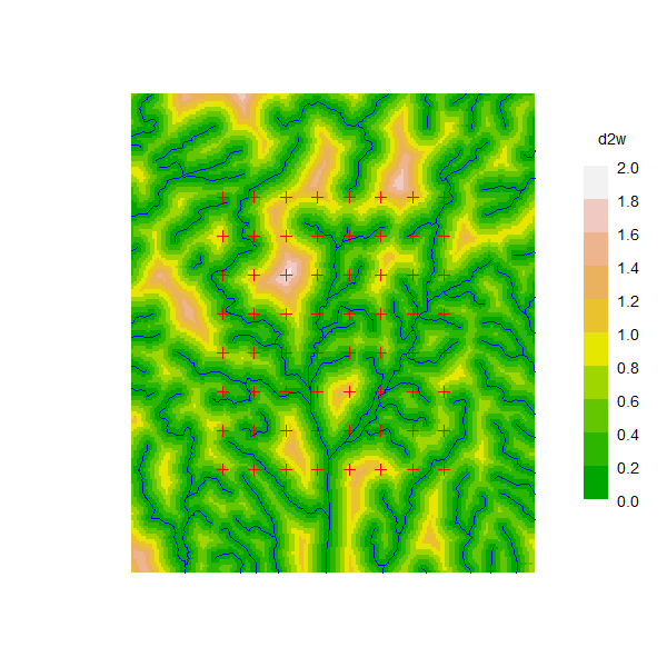

par(mar = c(1,6,1,6))
plot(sw2Dmask, covariate = "d2w", dots = FALSE)
plot(tr, add = TRUE)
plot(rivers, add = TRUE, col = "blue")

Figure F.4: Shaded plot of distance to water (d2w in km) with detector sites (red crosses) and rivers superimposed. Detector spacing 1.5 km N-S.

The distance function requires a value of the friction parameter ‘noneuc’ for each mask pixel. Distances are approximated using gdistance functions as before, except that we interpret the distance-to-water scale as ‘friction’ and invert that for gdistance.

dfn <- function (xy1, xy2, mask) {
    if (missing(xy1)) return("noneuc")
    require(gdistance)
    Sraster <- raster(mask, "noneuc")
    # conductance is inverse of friction
    trans <- transition(Sraster, transitionFunction = 
        function(x) 1/mean(x), directions = 16)
    trans <- geoCorrection(trans)
    costDistance(trans, as.matrix(xy1), as.matrix(xy2))
}    

The Royle et al. (2013) and Sutherland et al. (2015) models use an (\alpha_0, \alpha_1) parameterisation instead of (\lambda_0, \sigma). Their \alpha_2 translates directly to a coefficient in the secr model, as we’ll see. We consider just one realisation of one scenario (the package secrdesign Efford (2023) manages replicated simulations of multiple scenarios).

# parameter values from Sutherland et al. 2014
alpha0 <- -1   # implies lambda0 = invlogit(-1) = 0.2689414
sigma <- 1400
alpha1 <- 1 / (2 * sigma^2)
alpha2 <- 5    # just one scenario from the range 0..10
K  <- 10       # sampling over 10 occasions, collapsed to 1 occ

Now we are ready to build a simulated dataset.

# simulate fixed population of 200 animals in masked area
pop <- sim.popn (D = 200/nrow(sw2Dmask), core = tr, 
                 buffer = 3950, Ndist = "fixed")  
# to simulate non-Euclidean detection we attach a mask with 
# the pixel-specific friction to the simulated popn object
covariates(sw2Dmask)$noneuc <- exp(alpha2 * 
                                    covariates(sw2Dmask)$d2w)
attr(pop, "mask") <- sw2Dmask
# simulate detections, specifying non-Euclidean distance function
CH <- sim.capthist(tr, pop = pop, userdist = dfn, 
    noccasions = 1, binomN = K, detectpar = list(lambda0 = 
    invlogit(alpha0), sigma = sigma), detectfn = "HHN")

summary(CH, moves = TRUE)

Object class       capthist 
Detector type      count 
Detector number    64 
Average spacing    1385.7 m 
x-range            1698699 1708399 m 
y-range            2387891 2398391 m 

Counts by occasion 
                    1 Total
n                  37    37
u                  37    37
f                  37    37
M(t+1)             37    37
losses              0     0
detections        109   109
detectors visited  33    33
detectors used     64    64

Number of movements per animal
 0  1  2  3 
16 13  7  1 

Distance moved, excluding zero (m)
   Min. 1st Qu.  Median    Mean 3rd Qu.    Max. 
   1386    1386    1443    1552    1500    3151 

Individual covariates
 sex   
 F:21  
 M:16  

Model fitting is simple, but the default starting value for noneuc is not suitable and is overridden:

fitne1 <- secr.fit (CH, mask = sw2Dmask, detectfn = "HHN", 
    binomN = 10, model = noneuc ~ d2w -1, details = list(
    userdist = dfn), start = list(D = 0.005, lambda0 = 0.3,
    sigma = 1000, noneuc = 100), trace = FALSE)

The warning from nlm indicates a potential problem, but the standard errors and confidence limits below look plausible (they could be checked by running secr.refit with method = “none”). Fitting is slow (4 minutes on an aging PC). This is partly because the mask is large (32384 pixels) in order to maintain resolution in relation to the stream network.

coef(fitne1)

              beta  SE.beta     lcl      ucl
D          -5.3042 0.181714 -5.6603 -4.94800
lambda0    -1.1386 0.169830 -1.4715 -0.80577
sigma       7.1491 0.091395  6.9699  7.32821
noneuc.d2w  4.5961 0.503034  3.6102  5.58205

predict(fitne1)

        link   estimate SE.estimate        lcl        ucl
D        log 4.9709e-03  9.1079e-04 3.4814e-03 7.0976e-03
lambda0  log 3.2026e-01  5.4784e-02 2.2958e-01 4.4674e-01
sigma    log 1.2729e+03  1.1658e+02 1.0642e+03 1.5226e+03
noneuc   log 7.5395e+00  1.6876e+00 4.8881e+00 1.1629e+01

region.N(fitne1)

    estimate SE.estimate    lcl    ucl  n
E.N   160.98      29.495 112.74 229.85 37
R.N   160.98      26.627 118.77 224.97 37

The coefficient noneuc.d2w corresponds to alpha2. Estimates of predicted (‘real’) parameters D and lambda0, and the coefficient noneuc.d2w, and are comfortably close to the true values, and all true values are covered by the 95% CI.

We fit the ‘noneuc’ (friction) parameter through the origin (zero intercept; -1 in formula). The predicted value of ‘noneuc’ relates to the covariate value for the first pixel in the mask (d2w = 1.133 km), but in this zero-intercept model the meaning of ‘noneuc’ itself is obscure. In effect, the parameter alpha1 (or sigma) serves as the intercept; the same model may be fitted by fixing sigma (fixed = list(sigma = 1)) and estimating an intercept for noneuc (model = noneuc ~ d2w). In this case, ‘noneuc’ may be interpreted as the site-specific sigma (see also examples in the main text).

It is interesting to plot the predicted detection probability under the simulated model. For plotting we add the pdot value as an extra covariate of the mask. Note that pdot here uses the ‘noneuc’ value previously added as a covariate to sw2Dmask.

covariates(sw2Dmask)$predicted.pdot <- pdot(sw2Dmask, tr, 
    noccasions = 1, binomN = 10, detectfn = "HHN", detectpar = 
    list(lambda0 = invlogit(-1), sigma = sigma), userdist = dfn)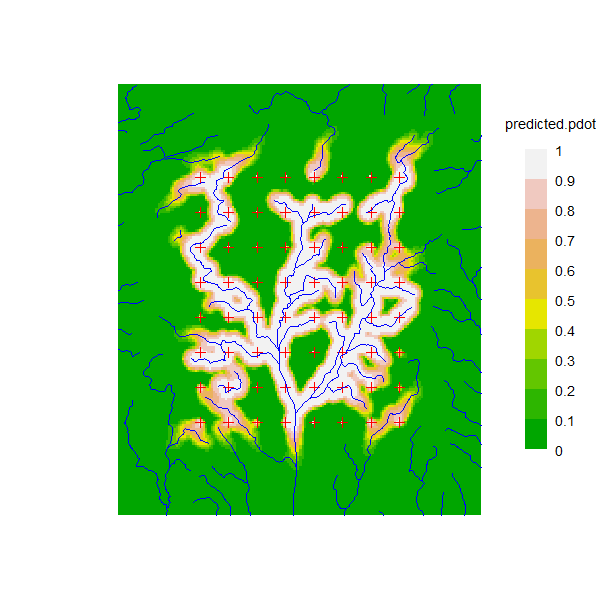

par(mar = c(1,6,1,6))
plot(sw2Dmask, covariate = "predicted.pdot", dots = FALSE)
plot(tr, add = TRUE)
plot(rivers, add = TRUE, col = "blue")

Figure F.5: Shaded plot of probability animal is detected at least once. Animals living within the detector array and away from a river (about half the population within the array) stand very little chance of being detected because the model confines them to a small home range and lambda0 is constant.

Borchers, D. L., & Kidney, D. (2014). Flexible density surface estimation for spatially explicit capture–recapture surveys. University of St Andrews. https://research-repository.st-andrews.ac.uk/bitstream/handle/10023/9147/secrgam_techrep.pdf?sequence=1

Csardi, G., & Nepusz, T. (2006). The igraph software package for complex network research. InterJournal, 1695. http://igraph.org

Efford, M. G. (2014). Bias from heterogeneous usage of space in spatially explicit capture-recapture analyses. Methods in Ecology and Evolution, 5, 599–602.

Efford, M. G. (2023). secrdesign: Sampling Design for Spatially Explicit Capture-Recapture. https://CRAN.R-project.org/package=secrdesign

Efford, M. G., Dawson, D. K., Jhala, Y. V., & Qureshi, Q. (2016). Density-dependent home-range size revealed by spatially explicit capture-recapture. Ecography, 39, 676–688.

Efford, M. G., & Mowat, G. (2014). Compensatory heterogeneity in spatially explicit capture-recapture data. Ecology, 95, 1341–1348.

Kendeigh, S. C. (1944). Measurement of bird populations. Ecological Monographs, 14, 67–106. https://doi.org/10.2307/1961632

Mowat, G., & Strobeck, C. (2000). Estimating population size of grizzly bears using hair capture, DNA profiling, and mark-recapture analysis. Journal of Wildlife Management, 64, 183–193.

Royle, J. A., Chandler, R. B., Gazenski, K. D., & Graves, T. A. (2013). Spatial capture-recapture models for jointly estimating population density and landscape connectivity. Ecology, 94, 287–294.

Sutherland, C., Fuller, A. K., & Royle, J. A. (2015). Modelling non-euclidean movement and landscape connectivity in highly structured ecological networks. Methods in Ecology and Evolution, 6, 169–177.

van Etten, J. (2023). Gdistance: Distances and routes on geographical grids. https://CRAN.R-project.org/package=gdistance

---

1. Mixing 2-km and 0.5-km cells carries a slight penalty: the centres of a few 2-km cells (<1%) do not lie in valid 0.5-km cells; these become inaccessible (infinite distance from all detectors) and are silently dropped in a later step.