ovenlist <- secrlist(ovenbird.model.1, ovenbird.model.D) 13 Working with fitted models
This chapter covers a miscellany of issues that arise regardless of the particular model to be fitted.
13.1 Bundling fitted models
You may have fitted one model or several. A convenient way to handle several models is to bundle them together as an object of class ‘secrlist’:
Most of the following functions accept both ‘secr’ and ‘secrlist’ objects. The multi-model fitting function list.secr.fit returns an secrlist.
13.2 Recognizing failure-to-fit
Sometimes a model may appear to have fitted, but on inspection some values are missing or implausible (near zero or very large). The maximization function nlm may return the arcane ‘code 3’, or there may be message that a variance calculation failed.
These conditions must be taken seriously, but they are not always fatal to the analysis. See Appendix A for diagnosis and possible solutions.
If all variances (SE) are missing or extreme then the fit has indeed failed.
13.3 Prediction
A fitted model (‘secr’ object) contains estimates of the coefficients of the model. Use the coef method for secr objects to display the coefficients (e.g., coef(secrdemo.0)). We note
- the coefficients (aka ‘beta parameters’) are on the link scale, and at the very least must be back-transformed to the natural scale, and
- a real parameter for which there is a linear sub-model is not unique: it takes a value that depends on covariates and other predictors.
These complexities are handled by the predict method for secr objects, as for other fitted models in R (e.g., lm). The desired levels of covariates and other predictors appear as columns of the ‘newdata’ dataframe. predict is called automatically when you print an ‘secr’ object by typing its name at the R prompt.
predict is commonly called with a fitted model as the only argument; then ‘newdata’ is constructed automatically by the function makeNewData. The default behaviour is disappointing if you really wanted estimates for each level of a predictor. This can be overcome, at the cost of more voluminous output, by setting all.levels = TRUE, or simply all = TRUE. For more customised output (e.g., for a particular value of a continuous predictor), construct your own ‘newdata’.
Density surfaces are a special case. Prediction across space requires the function predictDsurface as covered in Chapter 11.
13.4 Tabulation of estimates
The collate function is a handy way to assemble tables of coefficients or estimates from several fitted models. The input may be individual models or an secrlist. The output is a 4-dimensional array, typically with dimensions corresponding to
- session
- model
- statistic (estimate, SE, lcl, ucl)
- parameter (D, g0, sigma)
The parameters must be common to all models.
# [1,,,] drops 'session' dimension for printing
collate(secrdemo.0, secrdemo.CL, realnames = c('g0','sigma'))[1,,,]
, , g0
estimate SE.estimate lcl ucl
secrdemo.0 0.27319 0.027051 0.22348 0.32927
secrdemo.CL 0.27319 0.027051 0.22348 0.32927
, , sigma
estimate SE.estimate lcl ucl
secrdemo.0 29.366 1.3049 26.918 32.037
secrdemo.CL 29.366 1.3050 26.918 32.037Here we see that the full- and conditional-likelihood fits produce identical estimates for the detection parameters of a Poisson model.
13.5 Population size
The primary abundance parameter in secr is population density D. However, population size, the expected number of AC in a region A, may be predicted from any fitted model that includes D as a parameter.
Function region.N calculates \hat N(A) along with standard errors and confidence intervals (Efford & Fewster, 2013). The default region is the mask used to fit the model, but this is generally arbitrary, as we have seen, and users would be wise to specify the ‘region’ argument explicitly.
For an example of region.N in action, consider a model fitted to data on black bears from DNA hair snags in Great Smoky Mountains National Park, Tennessee.
code to fit black bear model
msk <- make.mask(traps(blackbearCH), buffer = 6000, type = 'trapbuffer',
                 poly = GSM, keep.poly = FALSE)  # clipped to park boundary
bbfit <- secr.fit(blackbearCH, model = g0~bk, mask = msk, trace = FALSE)
The region defaults to the extent of the original habitat mask:
region.N(bbfit) estimate SE.estimate lcl ucl n
E.N 444.6 55.003 349.19 566.07 139
R.N 444.6 50.801 360.11 561.36 139The two output rows relate to the ‘expected’ and ‘realised’ numbers of AC in the region. The distinction between expected (random) N and realised (fixed) N is explained by Efford & Fewster (2013). Typically the expected and realised N(A) from region.N are the same or nearly so, but deviations occur when the density model is not uniform. The estimated sampling error is less for ‘realised’ N(A) as part is fixed at the observed n.
The nominated region is arbitrary. It may be a new mask with different extent and cell size. If the model used spatial covariates the covariates must also be present in the new mask. If the density model did not use spatial covariates then the region may be a simple polygon.
It is interesting to extrapolate the number of black bears in the entire park (Fig. 13.1):
region.N(bbfit, region = GSM) estimate SE.estimate lcl ucl n
E.N 2091.9 258.80 1643.0 2663.5 139
R.N 2091.4 254.72 1652.5 2657.6 139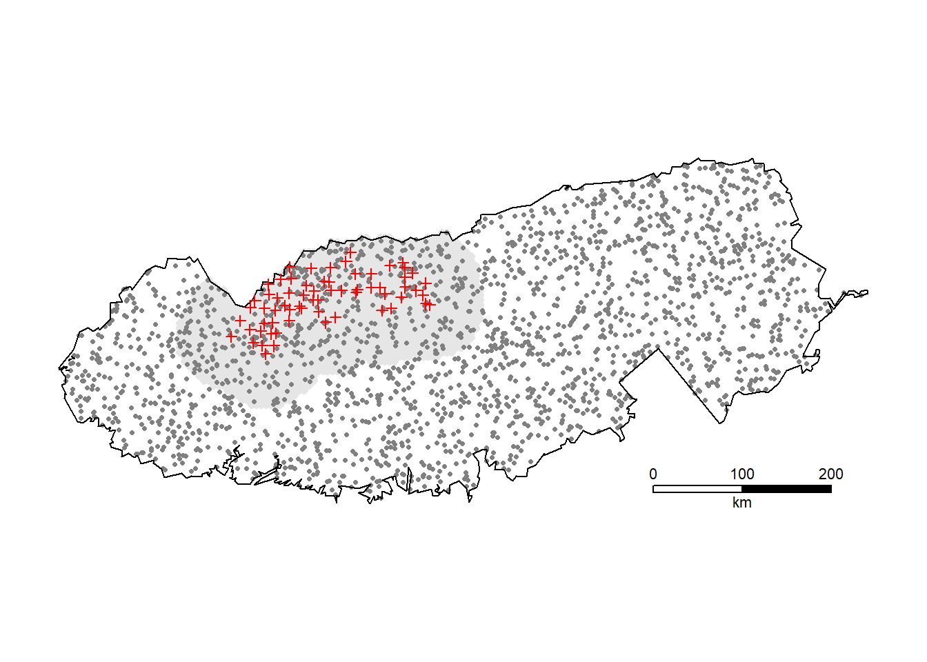
Estimates of realised population size (but not expected population size) are misleading if the new region does not cover all n detected animals.
13.6 Model selection
The best model is not necessarily the one that most closely fits the data. We need a criterion that penalises unnecessary complexity. For models fitted by maximum likelihood, the obvious and widely used candidate is Akaike’s Information Criterion AIC
\mathrm{AIC} = -2\log[L(\hat \theta)] +2K where K is the number of coefficients estimated and \log[L(\hat \theta)] is the maximized log likelihood.
Burnham & Anderson (2002), who popularised information-theoretic model selection for biologists, advocated the use of a small-sample adjustment due to Hurvich & Tsai (1989), designated AICc:
\mathrm{AIC}_c = -2\log(L(\hat{\theta})) + 2K + \frac{2K(K+1)}{n-K-1}.
Here we assume the sample size n is the number of individuals observed at least once (i.e. the number of rows in the capthist). This is somewhat arbitrary, and a reason to question the routine use of AICc. The additional penalty has the effect of decreasing the attractiveness of models with many parameters. The effect is especially large when n<2K.
Model selection by information-theoretic methods is open to misinterpretation. We do not attempt here to deal with the many subtleties, but raise some caveats:
Models to be compared by AIC must be based on identical data. Some options in
secr.fitsilently change the structure of the data and make models incompatible (‘CL’, ‘fastproximity’, ‘groups’, ‘hcov’, ‘binomN’). Comparisons should be made only within the family of models defined by constant settings of these options. A check of compatibility (standalone functionAICcompatible) is applied automatically in secr, but this is not guaranteed to catch all misuse.AICc is widely used. However, there are doubts about the correct sample size for AICc, and AIC may be a better basis for model averaging, as demonstrated by simulation for generalised linear models (Fletcher, 2019, p. 60). We use AIC in this book.
AIC values indicate the relative performance of models. Reporting AIC values per se is not helpful; present the differences \Delta \mathrm{AIC} between each model and the ‘best’ model.
13.6.1 Model averaging
Model weights may be used to form model-averaged estimates of real or beta parameters with modelAverage (see also Buckland et al. (1997) and Burnham & Anderson (2002)). Model weights are calculated as
w_i = \frac{\exp(-\Delta_i / 2),}{\sum{\exp(-\Delta_i / 2)}}, where \Delta refers to differences in AIC or AICc.
Models for which \Delta_i exceeds an arbitrary limit (e.g., 10) are given a weight of zero and excluded from the summation.
13.6.2 Likelihood ratio
If you have only two models, one a more general version of the other, then a likelihood-ratio test is appropriate. Here we compare an ovenbird model with density constant over time to one with a log-linear trend over years.
LR.test(ovenbird.model.1, ovenbird.model.D)
    Likelihood ratio test for two models

data:  ovenbird.model.1 vs ovenbird.model.D
X-square = 0.83, df = 1, p-value = 0.36
There is no evidence of a trend.
13.6.3 Model selection strategy
It is almost impossible to fit and compare all plausible SECR models. A strategy is needed to find a path through the possibilities. However, the available strategies are ad hoc and we cannot offer strong, evidence-based advice.
One strategy is to determine the best model for the detection process before proceeding to consider models for density. This is intuitively attractive.
Doherty et al. (2010) used simulation to assess model selection strategies for Cormack-Jolly-Seber survival analysis. They reported that the choice of strategy had little effect on bias or precision, but could affect model weights and hence affect model-averaged estimates.
We are not aware of any equivalent study for SECR.
13.6.4 Score tests
Models must usually be fitted to compare them by AIC. Score tests allow models at the next level in a tree of nested models to be assessed without fitting (McCrea & Morgan, 2011). Only the ‘best’ model at each level is fitted, perhaps spawning a further set of comparisons. This method is provided in secr (see ?score.test), but it has received little attention and its limits are unknown.
13.7 Assessing model fit
Rigor would seem to require that a model used for inference has been shown to fit the data. This premise has many fishhooks. Tests of absolute ‘goodness-of-fit’ for SECR have uniformly low power. Assumptions are inevitably breached to some degree, and we rely in practice on soft criteria (experience, judgement and the property of robustness) as covered in Chapter 6, and the relative fit of plausible models (indicated by AIC or similar criteria).
Nevertheless, tests of goodness-of-fit are potentially informative regarding ways a model might be improved. Early maximum likelihood and Bayesian approaches to SECR spawned different approaches to goodness-of-fit testing - the parametric bootstrap and Bayesian p-values. We present these in an updated context as this is an area of active research. Each test is introduced, along with a recent approach that attempts to bridge the divide by emulating Bayesian p-values for models fitted by maximum likelihood.
13.7.1 Parametric bootstrap
If an SECR model fits a dataset then a goodness-of-fit statistic computed from the data will lie close to the median of that statistic from replicated Monte Carlo simulations. Borchers & Efford (2008), following an earlier edition of Cooch & White (2023), suggested using a test based on the scaled deviance i.e. [-2\mathrm{log}{\hat L} + 2 \mathrm{log}L_{sat}] / \Delta df where \hat L is the likelihood evaluated at its maximum, L_{sat} is the likelihood of the saturated model (Table 13.1), and \Delta df is the difference in degrees of freedom between the two. The distribution of the test statistic was estimated by a parametric bootstrap i.e. by simulation from the fitted model with parameters fixed at the MLE.
| Model | Likelihood of saturated model |
|---|---|
| conditional | \log (n!) - \sum_\omega \log(n_\omega!) + \sum_\omega n_\omega \log(\frac{n_\omega}{n}) |
| Poisson | n\log(n) - n - \sum_\omega \log(n_\omega!) + \sum_\omega n_\omega \log(\frac{n_\omega}{n}) |
| Binomial | n\log(\frac{n}{N}) - (N-n)\log(\frac{N-n}{N}) + \log(\frac{N!}{(N-n)!})- \sum_\omega \log(n_\omega!) + \sum_\omega n_\omega \log(\frac{n_\omega}{n}) |
Warning
Saturated likelihoods are shown in Table 13.1 for the simplest models. There may be complications for models with groups, individual covariates etc. (cf Cooch & White, 2023, Section 5.1).
13.7.2 Bayesian p-values
Royle et al. (2014) (pp. 232–243) treated the problem of assessing model fit in the context of Bayesian SECR using Bayesian p-values (Gelman & Stern, 1996).
In essence, Bayesian p-values compare two discrepancies: the discrepancy between the observed and expected values, and the discrepancy between simulated and expected values. A discrepancy is a scalar summary statistic for the match between two sets of counts; Royle et al. (2014) used the Freeman-Tukey statistic (e.g., Brooks & Morgan, 2000) in preference to the conventional Pearson statistic. The statistic has this general form for M counts y_m with expected value \mathrm{E}(y_m): T = \sum_m \left[\sqrt {y_m} - \sqrt{E(y_m)}\right]^2.
Each pair of discrepancy statistics provides a binary outcome (Was the observed discrepancy greater than the simulated discrepancy?) and these are summarised as a ‘Bayesian p value’ i.e. the proportion of replicates in which the observed discrepancy exceeds the simulated discrepancy. The p value is expected to be around 0.5 for a model that fits.
13.7.3 Emulation of Bayesian p values
Choo et al. (2024) proposed novel simulation-based tests for SECR models fitted by maximum likelihood. Their idea was to emulate Bayesian p values by repeatedly –
- resampling density and detection parameters from a multivariate normal distribution based on the estimated variance-covariance matrix
- conditioning on the known (detected individuals) and locating each according to its post-hoc probability distribution (fxi in secr), using the resampled detection parameters
- simulating additional individuals from the post-hoc distribution of unobserved individuals, as required to make up the resampled density, also using the resampled detection parameters
- computing the expected values of chosen summary statistics (e.g. margins of the capthist array)
- computing two discrepancy statistics (e.g. Freeman-Tukey) for each realisation: observed vs expected and simulated vs expected.
The explicit ‘point of difference’ of the Choo et al. (2024) approach is the propagation of uncertainty in the parameter values instead of relying on the central estimates for a parametric bootstrap. This alone would not be expected to increase the power of the test over a conventional test, and might even reduce power. However, the comparison of observed vs expected and simulated vs expected is performed separately for each realisation of the parameters, including the distribution of AC, and this may add power (think of a paired t-test).
13.7.4 Implementation in secr
The parametric bootstrap is implemented in secr.test and the Choo et al. (2024) emulation of Bayesian p-values is implemented in MCgof. We have been unable to find a convincing application of goodness-of-fit to SECR data. Rather than promote either method we prefer to await developments.
13.8 Model re-fit
The fitting of a part-fitted model saved to a progress file may be resumed with secr.refit (Section 9.8.7.6). The function may also be used to re-fit a completed model, or to repeat just the variance estimation (Hessian) step.