12 Habitat mask
A mask represents habitat in the vicinity of detectors that is potentially occupied by the species of interest. Understanding habitat masks and how to define and manipulate them is central to spatially explicit capture–recapture. This chapter summarises what users need to know about masks in secr. Early sections apply regardless of software.
12.1 Background
We start with an intuitive explanation of the need for habitat masks. Devices such as traps or cameras record animals moving in a general region. If the devices span a patch of habitat with a known boundary then we use a mask to define that geographical unit. More commonly, detectors are placed in continuous habitat and the boundary of the region sampled is ill-defined. This is because the probability of detecting an animal tapers off gradually with distance.
Vagueness regarding the region sampled is addressed in spatially explicit capture–recapture by considering a larger and more inclusive region, the habitat mask. Its extent is not critical, except that it should be at least large enough to account for all detected animals.
Next we refine this intuitive explanation for each of the dominant methods for fitting SECR models: maximum likelihood and Markov-chain Monte Carlo (MCMC) sampling. Each grapples in a slightly different way with the awkward fact that, although we wish to model detection as a function of distance from the activity centre, the activity centre of each animal is at an unknown location.
12.1.1 Maximum likelihood and the area of integration
The likelihood developed for SECR by Borchers & Efford (2008) allows for the unknown centres by numerically integrating them out of the likelihood (crudely, by summing over all possible locations of detected animals, weighting each by a detection probability). Although the integration might, in principle, have infinite spatial bounds, it is practical to restrict attention to a smaller region, the ‘area of integration’. As long as the probability weights get close to zero before we reach the boundary, we don’t need to worry too much about the size of the region.
In secr the habitat mask equates to the area of integration: the likelihood is evaluated by summing values across a fine mesh of points. This is the primary function of the habitat mask; we consider other functions in Section 12.2.
12.1.2 MCMC and the Bayesian ‘state space’
MCMC methods for spatial capture–recapture developed by Royle and coworkers (Royle et al., 2014) take a slightly different tack. The activity centres are treated as a large number of unobserved (latent) variables. The MCMC algorithm ‘samples’ from the posterior distribution of location for each animal, whether detected or not. The term ‘state space’ is used for the set of permitted locations; usually this is a continuous (not discretized) rectangular region.
12.2 What is a mask for?
Masks serve multiple purposes in addition to the basic one we have just introduced. We distinguish five functions of a habitat mask and there may be more:
To define the outer limit of the area of integration. Habitat beyond the mask may be occupied, but animals centred there have negligible chance of being detected.
To facilitate computation. By defining the area of integration as a list of discrete points (the centres of grid cells, each with notionally uniform density) we transform the relatively messy task of numerical integration into the much simpler one of summation.
To distinguish habitat sites from non-habitat sites within the outer limit. Habitat cells have the potential to be occupied. Treating non-habitat as if it is habitat can cause habitat-specific density to be underestimated.
To store habitat covariates for spatial models of density. Covariates for modelling a density surface are provided for each point on the mask.
To define a region for which a post-hoc estimate of population size is required. This may differ from the mask used to fit the model.
The first point raises the question of where the outer limit should lie (i.e., the buffer width), and the second raises the question of how coarse the discretization (i.e., the cell size) can be without damaging the estimates. Later sections address each of the five points in turn, after an introductory section describing the particular implementation of habitat masks in the R package secr.
12.3 Masks in secr
A habitat mask is represented in secr by a set of square grid cells. Their combined area may be almost any shape and may include holes. An object of class ‘mask’ is a 2-column dataframe with additional attributes (cell area etc.); each row gives the x- and y-coordinates of the centre of one cell.
12.3.1 Masks generated automatically by secr.fit
A mask is used whenever a model is fitted with the function secr.fit, even if none is specified in the ‘mask’ argument. When no mask is provided, one is constructed automatically using the value of the ‘buffer’ argument. For example
The mask is saved as a component of the fitted model (‘secr’ object); we can plot it and overlay the traps:
code to plot automatically generated mask
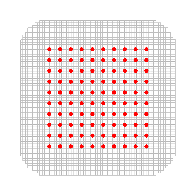
secr.fit by buffering around the detectors (red dots) (80-m buffer, 30-m detector spacing)
The mask is generated by forming a grid that extends ‘buffer’ metres north, south, east and west of the detectors and dropping centroids that are more than ‘buffer’ metres from the nearest detector (hence the rounded corners). The obvious question “How wide should the buffer be?” is addressed in a later section. The spacing of mask points (i.e. width of grid cells) is set arbitrarily to 1/64th of the east-west dimension - in this example the spacing is 6.7 metres.
12.3.2 Masks constructed with make.mask
A mask may also be prepared in advance and provided to secr.fit in the ‘mask’ argument. This overrides the automatic process of the preceding section, and the value of ‘buffer’ is discarded. The function make.mask provides precise control over the the size of the cells, the extent of the mask, and much more. We introduce make.mask here with a simple example based on a ‘hollow grid’:
code to plot mask from make.mask
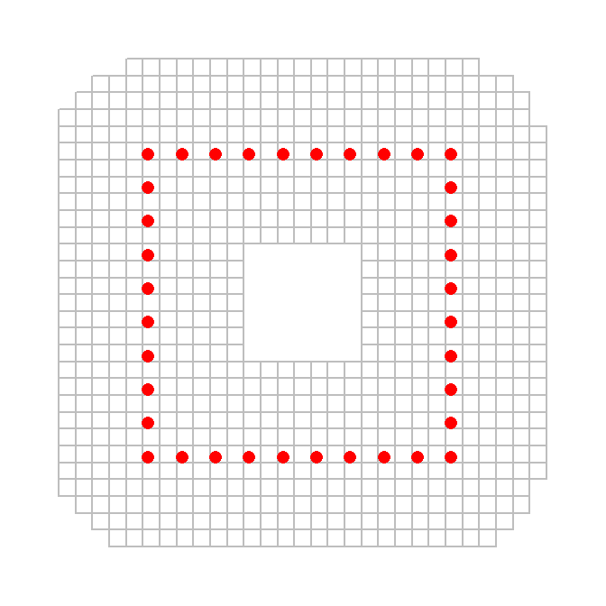
make.mask (80-m buffer, 30-m trap spacing, 15-m mask spacing). Grid cells in the centre were dropped because they were more than 80 m from any trap.
We chose a coarser grid (spacing 15 metres) relative to the trap spacing. This, combined with the hole in the centre, results in a mask with many fewer rows (764 rows compared to 3980). Setting the type to “trapbuffer” trims grid cells from the corners and the centre.
If we collected data hollowCH with the hollow grid we could fit a SECR model using hollowmask. For illustration we simulate some data using default settings in sim.capthist (5 occasions, D = 5/ha, g0 = 0.2, sigma = 25 m).
hollowCH <- sim.capthist(hollowgrid, seed = 123)
fit2 <- secr.fit(hollowCH, mask = hollowmask, trace = FALSE)
predict(fit2)
link estimate SE.estimate lcl ucl
D log 5.0807 1.078535 3.36683 7.66711
g0 logit 0.2047 0.044309 0.13117 0.30497
sigma log 26.1801 3.241670 20.55772 33.34021Fitting is fast because there are few traps and few mask points. As before, the mask is retained in the output, so –
12.4 How wide should the buffer be?
The general answer is ‘Wide enough that any bias in estimated densities is negligible’. Excessive truncation of the mask results in positive bias that depends on the sampling regime (detector layout and sampling duration) and the detection function, particularly its spatial scale and shape.
The penalty for using an over-wide buffer is that fitting will be slower for a given mask spacing. It is usually smart to accept this penalty rather than search for the narrowest acceptable buffer.
Two factors are critical when selecting a buffer width –
- The spatial scale of detection, which is usually a function of home-range movements.
- The shape of the detection function, particularly the length of its tail.
These must be considered together. The following comments assume the default half-normal detection function, which has a short tail and spatial scale parameter \sigma_{HN}, unless stated otherwise.
12.4.1 A rule of thumb for buffer width
As a rule of thumb, a buffer of 4\sigma_{HN} is likely to be adequate (result in truncation bias of less than 0.1%). A pilot estimate of \sigma_{HN} may be found for a particular dataset (capthist object) with the function RPSV with the argument ‘CC’ set to TRUE:
RPSV(captdata, CC = TRUE)[1] 25.629This is an approximation based on a circular bivariate normal distribution that ignores the truncation of recaptures due to the finite extent of the detector array (Calhoun & Casby, 1958).
12.4.2 Buffer width for heavy-tailed detection functions
Heavy-tailed detection functions such as the hazard-rate (HR, HHR) can be problematic because they require an unreasonably large buffer for stable density estimates. They are better avoided unless there is a natural boundary.
12.4.3 Hands-free buffer selection: suggest.buffer
The suggest.buffer function is an alternative to the 4\sigma_{HN} rule of thumb for data from point detectors (not polygon or transect detectors). It has the advantage of allowing for the geometry of the detector array (specifically, the length of edge) and the duration of sampling. The algorithm is obscure and undocumented (this is only a suggestion!) and uses an approximation to the bias, computed by function bias.D. The first argument of suggest.buffer may be a capthist object or a fitted model. With a capthist object as input:
suggest.buffer(captdata, detectfn = 'HN', RBtarget = 0.001)Warning: using automatic 'detectpar' g0 = 0.2339, sigma = 30.75[1] 105When the input is only a capthist object, the suggested buffer width relies on an estimate of \sigma_{HN} that is itself biased (RPSV(captdata, CC=TRUE)). Section 12.4.4 shows how the suggested buffer width changes when we use a better estimate of \sigma_{HN}. Actual bias due to mask truncation will also exceed the target (RB = 0.1%) due to limitations of the ad hoc algorithm in bias.D.
12.4.4 Retrospective buffer checks
Once a model has been fitted with a particular buffer width or mask, the estimated detection parameters may be used to check whether the buffer width is likely to have resulted in mask truncation bias. We highlight two of these:
-
secr.fitautomatically checks a mask generated from its ‘buffer’ argument (i.e. when the ‘mask’ argument is missing), usingbias.Das insuggest.buffer. A warning is given when the predicted truncation bias exceeds a threshold. The threshold is controlled by the ‘biasLimit’ argument (default 0.01). To suppress the check set ‘biasLimit = NA’, or provide a pre-defined mask.
The check is performed by a cunning custom algorithm in function bias.D. This uses one-dimensional numerical integration of a polar approximation to site-specific detection probability, coupled to a 3-part linear approximation for the length of contours of distance-to-nearest-detector. The check cannot be performed for some detector types, and the embedded integration can give rise to cryptic error messages.
-
esaPlotprovides a quick visualisation of the change in estimated density as buffer width changes. It is a handy check on any fitted model, and may also be used with pilot parameter values. The name of the function derives from its reliance on calculation of the effective sampling area (esa or a(\hat \theta)).
fit <- secr.fit(captdata, buffer = 100, trace = FALSE)par(pty = "s", mar = c(4,4,2,2), mgp = c(2.5,0.8,0), las = 1)
esaPlot(fit, ylim = c(0,10))
abline(v = 4 * 25.6, col = "red", lty = 2)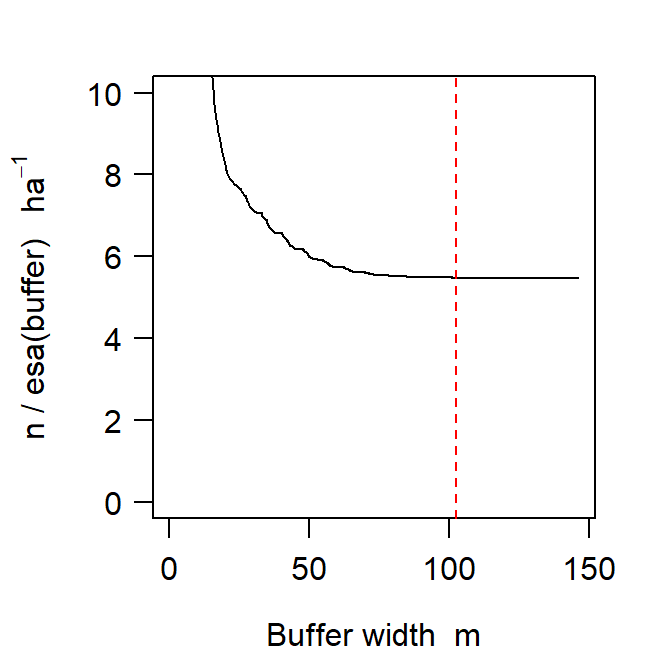
The esa plot supports the prediction that increasing buffer width beyond the rule-of-thumb value has no discernable effect on the estimated density (Fig. 12.3).
The function mask.check examines the effect of buffer width and mask spacing (cell size) by computing the likelihood or re-fitting an entire model. The function generates either the log likelihood or the estimated density for each cell in a matrix where rows correspond to different buffer widths and columns correspond to different mask spacings. The function is limited to single-session models and is slow compared to esaPlot. See ?mask.check for more.
Note also that suggest.buffer may be used retrospectively (with a fitted model as input), and
suggest.buffer(fit)[1] 100which is coincidental, but encouraging!
12.4.5 Buffer using non-Euclidean distances
If you intend to use a non-Euclidean distance metric then it makes sense to use this also when defining the mask, specifically to drop mask points that are distant from any detector according to the metric. See Appendix F for an example. Modelling with non-Euclidean distances also requires the user to provide secr.fit with a matrix of user-computed distances between detectors and mask points.
12.5 Grid cell size
Using a set of discrete locations (mask points) to represent the locations of animals is numerically convenient, and by making grid cells small enough we can certainly eliminate any effect of discretization. However, reducing cell size increases the number of cells and slows down model fitting. Trials with varying cell size (mask spacing) provide reassurance that discretization has not distorted the analysis.
In this section we report results from trials with four very different datasets for which details are given in the secr documentation: Maryland ovenbirds (ovenCH), Waitarere possums (possumCH), Arizona horned lizards (hornedlizardCH) and Tennessee black bears (blackbearCH). These studies used respectively mist nets, cage trapping, area search and DNA identification of hairs from barbed wire snares.
The reference scale was \sigma estimated earlier by fitting a half-normal detection model. In each case masks were constructed with constant buffer width 4\sigma and different spacings in the range 0.2\sigma to 3\sigma. This resulted in widely varying numbers of mask points (Fig. 12.4).
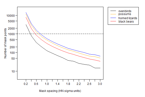
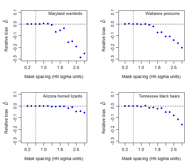
The results in Fig. 12.5 suggest that, for a uniform density model, any mask spacing less than the half-normal \sigma is adequate; 0.6\sigma provides a considerable safety margin. The effect of detector spacing on the relationship has not been examined. Referring back to Fig. 12.4, a mask of about 1000 points will usually be adequate with a 4\sigma buffer.
The default spacing in secr.fit and make.mask is determined by dividing the x-dimension of the buffered area by 64. The resulting mask typically has about 4000 points, which is overkill. Substantial improvements in speed can be obtained with coarser masks, obtained by reducing ‘nx’ or ‘spacing’ arguments of make.mask.
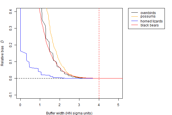
For completeness, we revisit the question of buffer width using the esaPlot function with each of the four test datasets (Fig. 12.6).
12.6 Excluding non-habitat
Our focus so far has been on choosing a buffer width to set the outer boundary of a habitat mask, assuming that the actual boundary is arbitrary. We can call these ‘masks of convenience’ (Fig. 12.7 a); numerical accuracy and computation speed are the only constraints. At the other extreme, a mask may represent a natural island of habitat surrounded by non-habitat (Fig. 12.7 c). A geographical map, possibly in the form of an ESRI shapefile, is then sufficient to define the mask. Between these extremes there are may be a habitat mosaic including both some non-habitat near the detectors and some habitat further away, so neither the buffered mask of convenience nor the habitat island is a good match (Fig. 12.7 b).
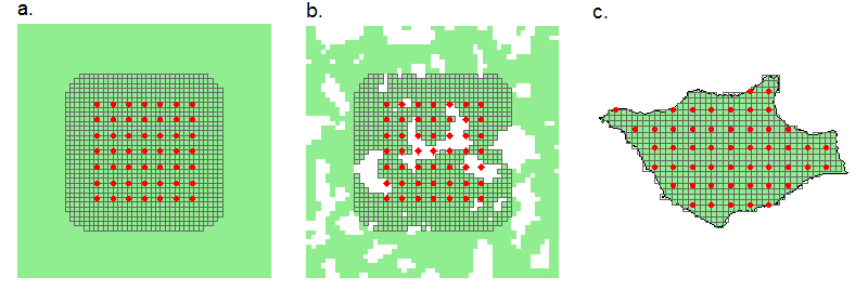
The virtue of clipping non-habitat is that the estimate of density then relates to the area of habitat rather than the sum of habitat and non-habitat. For most uses habitat-based density would seem the more meaningful parameter.
Exclusion of non-habitat (Fig. 12.7 b,c) is achieved by providing make.mask with a digital map of the habitat in the ‘poly’ argument. The digital map may be an R object defining spatial polygons as described in Appendix C, or simply a 2-column matrix or dataframe of coordinates. This simple example uses the coordinates in possumarea:
code to plot clipped mask
By default, data for the ‘poly’ argument are retained as an attribute of the mask. With some data sources this grossly inflates the size of the mask, and it is better to discard the attribute with keep.poly = FALSE.
12.7 Mask covariates
Masks may have a ‘covariates’ attribute that is a dataframe just like the ‘covariates’ attributes of traps and capthist objects. The data frame has one row for each row (point) on the mask, and one column for each covariate. The dataframe may include unused columns. Mask covariates are used for modelling [density surfaces] (D), not for modelling detection parameters (g0, lambda0, sigma).
Covariates may be categorical (factor-valued) or continuous. Character-valued covariates will be coerced to factors. Covariates in detection models ideally take a small number of discrete values, but there is no such constraint on mask covariates, which may be continuous.
12.7.1 Adding covariates
Mask covariates are always added after a mask is first constructed. Extending the earlier example, we can add a covariate for the computed distance to shore:
covariates(clippedmask) <- data.frame(d.to.shore =
    distancetotrap(clippedmask, possumarea))
The function addCovariates makes it easy to extract data for each mask cell from a spatial data source. Its usage is
addCovariates (object, spatialdata, columns = NULL,
    strict = FALSE, replace = FALSE)
Values are extracted for the point in the data source corresponding to the centre point of each grid cell. The spatial data source (spatialdata) should be one of
- ESRI polygon shapefile name (excluding .shp)
- sf spatial object, package sf
- RasterLayer, package raster
- SpatRaster, package terra
- SpatialPolygonsDataFrame, package sp
- SpatialGridDataFrame, package sp
- another mask with covariates
- a traps object with covariates
One or more input columns may be selected by name. The argument ‘strict’ generates a warning if points lie outside a mask used as a spatial data source. Appendix C has more about spatial data in secr.
See Chapter 11 for further applications, including smooths to represent the scale of effect.
12.7.2 Repairing missing values
Covariate values become NA for points not in the data source for addCovariates. Modelling will fail until a valid value is provided for every mask point (ignoring covariates not used in models). If only a few values are missing at only a few points it is usually acceptable to interpolate them from surrounding non-missing values. For continuous covariates we suggest linear interpolation with the function interp in the akima package (Akima & Gebhardt, 2022). The following short function provides an interface:
repair <- function (mask, covariate, ...) {
    NAcov <- is.na(covariates(mask)[,covariate])
    OK <- subset(mask, !NAcov)
    require(akima)
    irect <- akima::interp (x = OK$x, y = OK$y, z =
        covariates(OK)[,covariate],...)
    irectxy <- expand.grid(x = irect$x, y = irect$y)
    i <- nearesttrap(mask[NAcov,], irectxy)
    covariates(mask)[,covariate][NAcov] <- irect[[3]][i]
    mask
}
To demonstrate repair we deliberately remove a swathe of covariate values from a copy of our clippedmask and then attempt to interpolate them (Fig. 12.9):
damagedmask <- clippedmask
covariates(damagedmask)$d.to.shore[500:1000] <- NA
repaired <- repair(damagedmask, 'd.to.shore', nx=60, ny=50)
The interpolation may potentially be improved by varying the interp arguments nx and ny (passed via the … argument of repair). Although extrapolation is available (with linear = FALSE, extrap = TRUE) it did not work in this case, and there remain some unfilled cells (Fig. 12.9 c).
Categorical covariates pose a larger problem. Simply copying the closest valid value may suffice to allow modelling to proceed, and this is a good solution for the few NA cells in Fig. 12.9 c. The result should always be checked visually by plotting the covariate: strange patterns may result.
copynearest <- function (mask, cov) {
    NAcov <- is.na(covariates(mask)[,cov])
    OK <- subset(mask, !NAcov)
    i <- nearesttrap(mask, OK)
    covariates(mask)[,cov][NAcov] <- covariates(OK)[i[NAcov],cov]
    mask
}
completed <- copynearest(repaired, 'd.to.shore')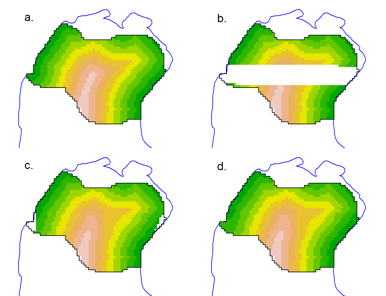
See Chapter 11 for more on the use of mask covariates.
12.8 Regional population size
Population density D is the primary parameter in this implementation of spatially explicit capture–recapture (SECR). The number of individuals (population size N(A)) is treated as a derived parameter. The rationale for this is that population size is ill-defined in many classical sampling scenarios in continuous habitat (Figs. 7a,b). Population size is well-defined for a habitat island (Fig. 12.7 c). Population size may also be well-defined for a persistent swarm, colony, herd, pack or flock, although group living is incompatible with the usual SECR assumption of independence e.g. Bischof et al. (2020).
Population size on a habitat island A may be derived from an SECR model by the simple calculation \hat N = \hat D|A| if density is uniform. The same calculation yields the expected population in any area A^\prime. Calculations get more tricky if density is not uniform as then \hat N = \int_{A^\prime} D(\mathbf x) \, d\mathbf x (computing the volume under the density surface) (Efford & Fewster, 2013). secr provides the function region.N for this purpose (Section 13.5).
12.9 Plotting masks
The default plot of a mask shows each point as a grey dot. We have used dots = FALSE throughout this document to emphasise the gridcell structure. That is especially handy when we use the plot method to display mask covariates:
par(mar = c(1,1,2,6), xpd = TRUE)
plot(clippedmask, covariate = 'd.to.shore', dots = FALSE,
    border=100, title = 'Distance to shore m', polycol = 'blue')
plotMaskEdge(clippedmask, add = TRUE)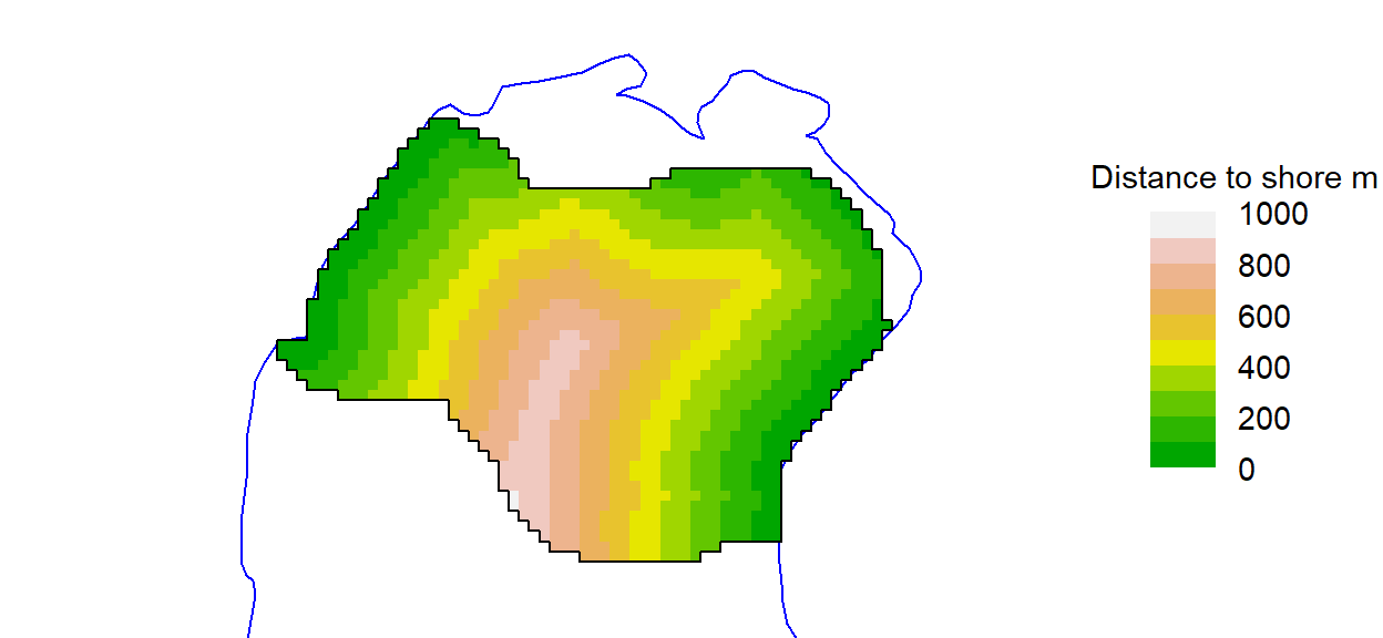
The legend may be suppressed with legend = FALSE. See ?plot.mask for details. We used plotMaskEdge to add a line around the perimeter.
12.10 More on creating and manipulating masks
12.10.1 Arguments of make.mask
The usage statement for make.mask is included as a reminder of various options and defaults that have not been covered in this vignette. See ?make.mask for details.
make.mask (traps, buffer = 100, spacing = NULL, nx = 64, ny = 64,
    type = c("traprect", "trapbuffer", "pdot", "polygon",
    "clusterrect", "clusterbuffer", "rectangular", "polybuffer"),
    poly = NULL, poly.habitat = TRUE, cell.overlap = c("centre",
    "any", "all"), keep.poly = TRUE, check.poly = TRUE,
    pdotmin = 0.001, random.origin = FALSE, ...)
12.10.2 Mask attributes saved by make.mask
Mask objects generated by make.mask include several attributes not usually on view. Use str to reveal them. Three are simply saved copies of the arguments ‘polygon’, ‘poly.habitat’ and ‘type’, and ‘covariates’ has been discussed already.
The attribute ‘spacing’ is the distance in metres between adjacent grid cell centres in either x- or y- directions.
The attribute ‘area’ is the area of a single grid cell in hectares (1 ha = 10000 m2, so area = spacing2 / 10000; retrieve with attr(mask, 'area')). Use the function maskarea to find the total area of all mask cells; for example, here is the area in hectares of the clipped Waitarere possum mask.
maskarea(clippedmask)[1] 205.06The attribute ‘boundingbox’ is a 2-column dataframe with the x- and y-coordinates of the corners of the smallest rectangle containing all grid cells.
The attribute ‘meanSD’ is a 2-column dataframe with the means and standard deviations of the x- and y-coordinates. These are used to standardize the coordinates if they appear directly in a model formula (e.g., D ~ x + y).
12.10.3 Linear habitat
Models for data from linear habitats analysed in the package secrlinear (Efford, 2024) use the class ‘linearmask’ that inherits from ‘mask’. Linear masks have additional attributes ‘SLDF’ and ‘graph’ to describe linear habitat networks. See [secrlinear-vignette.pdf] for details.
12.10.4 Dropping points from a mask
If the mask you want cannot be obtained directly with make.mask then use either subset (batch) or deleteMaskPoints (interactive; unreliable in RStudio). This ensures that the attributes are updated properly. Do not simply extract the required points from the mask dataframe by subscripting ([).
12.10.5 Multi-session masks
Fitting a SECR model to a multi-session capthist requires a mask for each session. If a single mask is passed to secr.fit then it will be replicated and must be appropriate for all sessions. The alternative is to provide a list of masks, one per session, in the correct order; make.mask generates such a list from a list of traps objects. See Chapter 14 for details.
12.10.6 Artificial habitat maps
Function randomHabitat generates somewhat realistic maps of habitat that may be used in simulations. It assigns mask pixels to ‘habitat’ and ‘non-habitat’ according to an algorithm that clusters habitat cells together. The classification is saved as a covariate in the output mask, from which non-habitat cells may be dropped entirely (this was used to generate the green habitat background in Fig. 12.7 b).
12.10.7 Mask vs raster
Mask objects have a lot in common with objects of the RasterLayer S4 class defined in the package raster (Hijmans, 2023a) and the SpatRaster class defined in the package terra (Hijmans, 2023b). However, they are much simpler: no projection is specified and grid cells must be square.
A mask object may be exported as a RasterLayer using the raster method defined in secr for mask objects. This allows you to nominate a covariate to provide values for the RasterLayer, and to specify a projection.
A mask object may also be exported as a SpatRaster using the rast method defined in secr for mask objects. See here for an example in which terra functions are used to smooth a mask covariate before returning it to the mask.
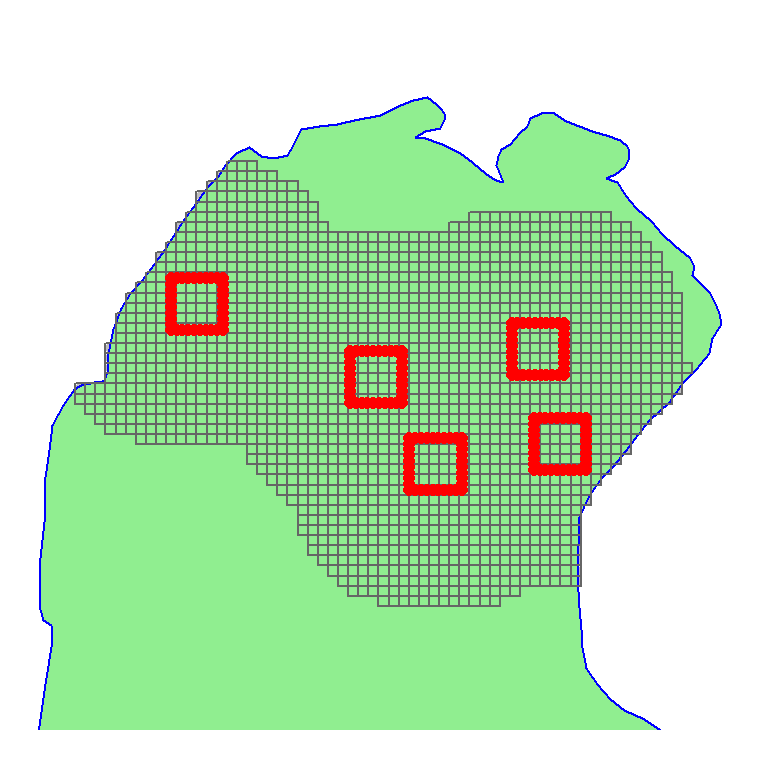
Inappropriate mask spacing is a common source of problems. Model fitting can be painfully slow if the mask has too many cells. Choose the spacing (cell size) as described in Grid cell size. A single mask for widely scattered clusters of traps should drop cells from wide inter-cluster spaces (set ‘type = trapbuffer’).