16  Sex differences

It is common for males and females to differ in their behaviour in relation to detectors. Sex is commonly recorded for trapped animals or those detected with automatic cameras, and hair samples used to identify individuals by their DNA can also reveal sex given suitable sex-specific markers. SECR models that allow for sex differences are therefore of particular interest.

There are many ways to model sex differences in secr, and each of these has already been mentioned in a general context. Here we enumerate the possibilities and comment on their usefulness.

Unlike some effects, the relevance of sex may be obvious from the beginning. You may therefore be happy to structure other aspects of the model around your chosen way to include sex. Alternately, other considerations may constrain the treatment of sex. The example below shows that several different ways of including sex lead to the same estimates.

16.1 Models

We list the possible models in order of usefulness (your mileage may vary; see also the decision chart below):

1. Hybrid mixture model
2. Conditional likelihood with individual covariate
3. Separate sessions
4. Full likelihood with groups

16.1.1 Hybrid mixtures

This method accommodates occasional missing values and estimates the sex ratio as a parameter (pmix). The method works for both conditional and full likelihood. If estimated (CL = FALSE) the absolute density D includes both classes. The sex ratio is estimated as a parameter (pmix).

16.1.2 Individual covariate

Including sex as an individual covariate in the model requires the model to be fitted by maximizing the conditional likelihood (CL = TRUE). Include a categorical (factor) covariate in model formulae (e.g., g0 \sim sex).

Tip

Derived densities are computed from a CL model with function derived. To get sex-specific densities specify groups = "sex" in derived.

16.1.3 Sex as session

It is possible to model data for the two sexes as different sessions (most easily, by coding ‘female’ or ‘male’ in the first column of the capture file read with read.capthist). Sex differences are then modelled by including a ‘session’ term in relevant model formulae (e.g., g0 \sim session).

Warning

Parameters not explicitly modelled as session-specific are assumed to be shared. In a full-likelihood model you also need D \sim session to allow for an uneven sex ratio.

16.1.4 Groups

Groups were described earlier. Use full likelihood (CL = FALSE), define groups = "sex" or similar, and include a group term ‘g’ in relevant formulae (e.g., g0 \sim g). ‘CL’ and ‘groups’ are arguments of secr.fit. The preceding Warning applies also to groups.

16.2 Demonstration

We re-analyse the morning house mouse data already analysed in Chapter 15. For all methods except the hybrid mixture we have to discard one individual of unknown sex (hence capthist marked with ‘x’). Close inspection of the results shows that the methods are equivalent.

morning <- subset(housemouse, occ = c(1,3,5,7,9)) # includes one mouse with sex unknown
morningx <- subset(housemouse, !is.na(covariates(housemouse)$sex), occ = c(1,3,5,7,9))
morningxs <- split(morningx, covariates(morningx)$sex)  # split into two sessions

# conditional likelihood
hybridxCL  <- secr.fit(morningx, model = list(lambda0~h2, sigma~h2),
                CL = TRUE, buffer = 25, detectfn = 'HEX', 
                trace = FALSE,  hcov = 'sex')
xCL        <- secr.fit(morningx, model = list(lambda0~sex, 
                sigma~sex), CL = TRUE, buffer = 25, detectfn = 'HEX', 
                trace = FALSE)
sessionxCL <- secr.fit(morningxs, model = list(lambda0~session, 
                sigma~session), CL = TRUE, buffer = 25, 
                detectfn = 'HEX', trace = FALSE)

fitsCL <- secrlist(hybridxCL,xCL,sessionxCL)
predict(fitsCL, all.levels = TRUE)

$hybridxCL
$hybridxCL$`session = coulombe, h2 = f`
         link estimate SE.estimate     lcl     ucl
lambda0   log  0.28819    0.041538 0.21758 0.38171
sigma     log  2.17887    0.153222 1.89866 2.50043
pmix    logit  0.46619    0.043007 0.38363 0.55064

$hybridxCL$`session = coulombe, h2 = m`
         link estimate SE.estimate     lcl     ucl
lambda0   log  0.20098    0.036023 0.14183 0.28478
sigma     log  2.05123    0.173554 1.73830 2.42051
pmix    logit  0.53381    0.043007 0.44936 0.61637


$xCL
$xCL$`session = coulombe, sex = f`
        link estimate SE.estimate     lcl     ucl
lambda0  log  0.28819    0.041539 0.21758 0.38171
sigma    log  2.17887    0.153222 1.89866 2.50043

$xCL$`session = coulombe, sex = m`
        link estimate SE.estimate     lcl     ucl
lambda0  log  0.20098    0.036023 0.14183 0.28478
sigma    log  2.05123    0.173555 1.73829 2.42051


$sessionxCL
$sessionxCL$`session = f`
        link estimate SE.estimate     lcl     ucl
lambda0  log  0.28818    0.041538 0.21758 0.38171
sigma    log  2.17887    0.153223 1.89866 2.50044

$sessionxCL$`session = m`
        link estimate SE.estimate     lcl     ucl
lambda0  log  0.20098    0.036023 0.14184 0.28478
sigma    log  2.05123    0.173554 1.73829 2.42050

# full likelihood
hybridx  <- secr.fit(morningx, model = list(lambda0~h2, sigma~h2), 
              hcov = 'sex', CL = FALSE, buffer = 25, detectfn = 'HEX', 
              trace = FALSE)
sessionx <- secr.fit(morningxs, model = list(D ~ session, 
              lambda0~session, sigma~session), CL = FALSE, buffer = 25,
              detectfn = 'HEX', trace = FALSE)
# suppress bias check that gives ignorable error in secr 5.2
groupx   <- secr.fit(morningx, model = list(D ~ g, lambda0~g, sigma~g), 
              groups = 'sex', CL = FALSE, buffer = 25, detectfn = 'HEX', 
              biasLimit = NA, trace = FALSE)

fits <- secrlist(hybridx,sessionx, groupx)
predict(fits, all.levels = TRUE)

$hybridx
$hybridx$`session = coulombe, h2 = f`
         link   estimate SE.estimate        lcl        ucl
D         log 1296.94081  112.480096 1094.55112 1536.75368
lambda0   log    0.28819    0.041538    0.21758    0.38171
sigma     log    2.17887    0.153221    1.89866    2.50043
pmix    logit    0.46619    0.043008    0.38363    0.55064

$hybridx$`session = coulombe, h2 = m`
         link   estimate SE.estimate        lcl        ucl
D         log 1296.94081  112.480096 1094.55112 1536.75368
lambda0   log    0.20098    0.036023    0.14183    0.28478
sigma     log    2.05123    0.173553    1.73830    2.42051
pmix    logit    0.53381    0.043008    0.44936    0.61637


$sessionx
$sessionx$`session = f`
        link  estimate SE.estimate       lcl       ucl
D        log 604.61389   72.458365 478.44449 764.05511
lambda0  log   0.28819    0.041538   0.21758   0.38171
sigma    log   2.17887    0.153221   1.89866   2.50043

$sessionx$`session = m`
        link  estimate SE.estimate       lcl       ucl
D        log 692.32722   86.800581 542.01062 884.33136
lambda0  log   0.20098    0.036023   0.14184   0.28478
sigma    log   2.05123    0.173551   1.73830   2.42050


$groupx
$groupx$`session = coulombe, g = f`
        link  estimate SE.estimate       lcl       ucl
D        log 604.61767   72.458613 478.44780 764.05939
lambda0  log   0.28819    0.041538   0.21758   0.38171
sigma    log   2.17886    0.153220   1.89866   2.50042

$groupx$`session = coulombe, g = m`
        link  estimate SE.estimate       lcl       ucl
D        log 692.32687   86.800590 542.01026 884.33104
lambda0  log   0.20098    0.036023   0.14183   0.28478
sigma    log   2.05123    0.173552   1.73830   2.42050

Execution time varies considerably:

Timing, conditional likelihood

 hybridxCL.elapsed        xCL.elapsed sessionxCL.elapsed 
              6.75               3.63              20.06 

Timing, full likelihood

 hybridx.elapsed sessionx.elapsed   groupx.elapsed 
            9.87            41.67             8.25 

16.3 Choosing a model

16.3.1 Sex-specific detection

We suggest the decision chart in Fig. 16.1. This omits ‘session’ approaches that we previously included for comparison, because they are rather slow and clunky and group models are equivalent.

Figure 16.1: Decision chart for including sex in detection model. `sexcov’ is a character value naming a 2-level character or factor individual covariate after some trial and error with out.width units etc.

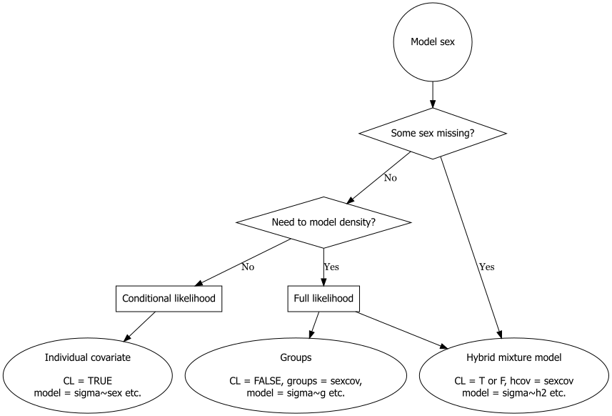
16.3.2 Sex-specific density

Fig. 16.1 is concerned solely with the detection model. Code for estimating sex-specific densities is available for each option as shown in Table 16.1. Sex ratio (pmix) is estimated directly only from hybrid mixture models. Post-hoc specification of ‘groups’ in derived works for both conditional and full likelihood models when density is constant. It is a common mistake to omit D~g or D~session from full-likelihood sex models – this forces a 1:1 sex ratio.

Table 16.1: Sex-specific estimates of density from various models. Any detection parameter may precede ‘~’

Fitting method	Model	Sex-specific density
Conditional likelihood	~sex1	derived(fit, groups = sexcov)
	~h2, hcov = sexcov	derived(fit, groups = sexcov)
	~session	derived(fit)
Full likelihood	D~g, ~g, groups = sexcov	predict(fit))
	~h2, hcov = sexcov	derived(fit, groups = sexcov)2
	D~session, ~session	predict(fit)

16.4 Final comments

We note

• Only hybrid mixtures can cope with missing values of the sex covariate.
• The implementation of groups is less comprehensive and may not be available for extensions in the Appendices.
• Options should not be mixed for comparing model fit by AIC.

Sex differences in home-range size (and hence \sigma) may be mitigated by compensatory variation in g_0 or \lambda_0 (Efford & Mowat, 2014) (see also Mitigating factors in Chapter 15).

Efford, M. G., & Mowat, G. (2014). Compensatory heterogeneity in spatially explicit capture-recapture data. Ecology, 95, 1341–1348.

Kendeigh, S. C. (1944). Measurement of bird populations. Ecological Monographs, 14, 67–106. https://doi.org/10.2307/1961632