9  R package secr

This chapter provides an overview of secr (Efford, 2025a). Following chapters expand on key topics.

To reproduce examples in the book you will need a recent version of secr (5.2.0 or later). Text in this font refers to R objects that are documented in online help for the secr package, or in base R. R code often generates warnings. Some warnings are merely reminders (e.g., that a default value is used for a key argument). For clarity, we do not display routine warnings for examples in the text.

In the examples we often use the function list.secr.fit to fit several competing models while holding constant other arguments of secr.fit. The result is a single ‘secrlist’ that may be passed to AIC, predict etc.

9.1 History

secr supercedes the Windows program DENSITY, an earlier graphical interface to SECR methods (Efford et al., 2004; Efford, 2012). The package was first released in March 2010 and continues to be developed. It implements almost all the methods described by Borchers & Efford (2008), Efford, Borchers, et al. (2009), Efford (2011), Efford & Fewster (2013), Efford et al. (2013), Efford & Mowat (2014), Efford et al. (2016), Efford & Hunter (2018) and Efford (2025b). External C++ code (Eddelbuettel et al., 2023) is used for computationally intensive operations. Multi-threading on multiple CPUs with RcppParallel (Allaire et al., 2023) gives major speed gains. The package is available from CRAN; the development version is on GitHub.

An interactive graphic user interface to many features of secr is provided by the Shiny app ‘secrapp’ available on GitHub and, currently, on a server at the University of Otago.

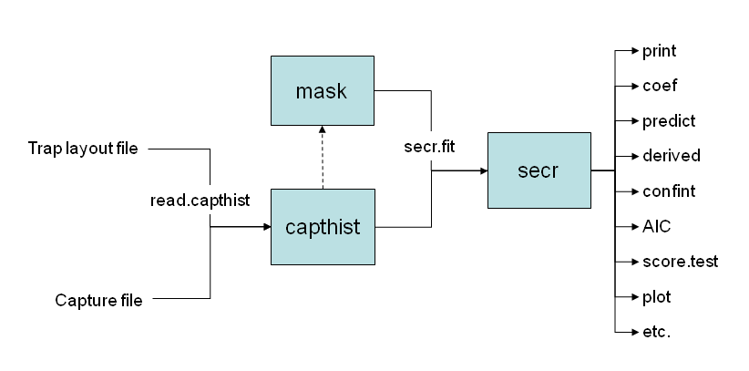
9.2 Object classes

R operates on objects each of which has a class. secr defines a set of R classes and methods for spatial capture–recapture data and models fitted to those data. To perform an SECR analysis you construct each of these objects in turn. Fig. 9.1 indicates the relationships among the classes.

R classes

A ‘class’ in R specifies a particular type of data object and the functions (methods) by which it is manipulated (computed, printed, plotted etc). Technically, secr uses old-fashioned ‘S3’ classes. See the R documentation ?class for further explanation.

Table 9.1: Essential classes in secr

Class	Data
traps	locations of detectors; detector type (‘proximity’, ‘multi’, etc.)
capthist	spatial detection histories, including a ‘traps’ object
mask	raster map of habitat near the detectors
secr	fitted SECR model

Figure 9.1: Workflow in secr

• Each object class (shaded box) comes with methods to display and manipulate the data it contains (e.g. print, summary, plot, rbind, subset).
• The function read.capthist forms a ‘capthist’ object from input in two files, one the detector layout (saved as attribute ‘traps’) and the other the capture data.
• By default, a habitat mask is generated automatically by secr.fit using a specified buffer around the detectors (traps) (dashed arrow). The function make.mask gives greater control over this step.
• Any of the objects input to secr.fit (traps, capthist, mask) may include a dataframe of covariates saved as an attribute. Covariate names may be used in model formulae; the covariates method is used to extract or replace covariates. Use addCovariates for trap or mask covariates from spatial data sources (e.g., shapefile or ‘sf’ object)
• Fitted secr models may be manipulated with the methods shown on the right.

Tip

Avoid using ‘[’ to extract subsets from capthist, traps, mask and other secr objects. Use the provided subset methods. It is generally safe to use ‘[[’ to extract one session from a multi-session capthist object.

9.3 Functions

For details of how to use each secr function see the help pages and vignettes.

Table 9.2: Core functions of secr. S3 methods are marked with an asterisk

Function	Purpose
addCovariates	add spatial covariates to traps or mask
AIC*	model selection, model weights
covariates	extract or replace covariates of traps, capthist or mask
derived*	compute density from conditional likelihood models
make.mask	construct habitat mask (= mesh)
plot*	plot capthist, traps or mask
predict*	compute ‘real’ parameters for arbitrary levels of predictor variables
predictDsurface	evaluate density surface at each point of a mask
read.capthist	input captures and trap layout from Density format, one call
region.N*	compute expected and realised population size in specified region
secr.fit	maximum likelihood fit; result is a fitted ‘secr’ object
summary*	summarise capthist, traps, mask, or fitted model
traps	extract or replace traps object in capthist

9.4 Detector types

Each ‘traps’ object has a detector type attribute that is a character value.

Table 9.3: Basic detector types in secr. See the appendices for area-search and telemetry types.

Name	Type	Description
“single”	single-catch trap	catch one animal at a time
“multi”	multi-catch trap	may catch more than one animal at a time
“proximity”	binary proximity	records presence at a point without restricting movement
“count”1	Poisson count proximity	[binomN = 0] allows >1 detection per animal per time
	Binomial count proximity	[binomN > 0] up to binomN detections per animal per time

1. The “count” detector type is generic for integer data; the actual type depends on the secr.fit argument ‘binomN’.

There is limited support in secr for the analysis of locational data from telemetry (‘telemetry’ detector type). Telemetry data are used to augment capture–recapture data (Appendix G).

9.5 Input

Data input is covered in the data input vignette secr-datainput.pdf. One option is to use text files in the formats used by DENSITY; these accommodate most types of data. Two files are required, one of detector (trap) coordinates and one of the detections (captures) themselves; the function read.capthist reads both files and constructs a capthist object. It is also possible to construct the capthist object in two stages, first making a traps object (with read.traps) and a captures dataframe, and then combining these with make.capthist. This more general route may be needed for unusual datasets.

9.6 Output

Function secr.fit returns an object of class secr. This is an R list with many components. Assigning the output to a named object saves both the fit and the data for further manipulation. Typing the object name at the R prompt invokes print.secr which formats the key results. These include the dataframe of estimates from the predict method for secr objects. Functions are provided for further computations on secr objects (e.g., AIC model selection, model averaging, profile-likelihood confidence intervals, and likelihood-ratio tests). Several of these were listed in Table 9.2.

One system of units is used throughout . Distances are in metres and areas are in hectares (ha). The unit of density for 2-dimensional habitat is animals per hectare. 1 ha = 10000 m² = 0.01 km². To convert density to animals per km², multiply by 100. Density in linear habitats (see package secrlinear) is expressed in animals per km.

9.7 Documentation and support

The primary documentation for secr is in the help pages that accompany the package. Help for a function is obtained in the usual way by typing a question mark at the R prompt, followed by the function name. Note the ‘Index’ link at the bottom of each help page – you will probably need to scroll down to find it. The index may also be accessed with help(package = secr). Static and potentially outdated versions of the help pages are available here.

The consolidated help pages are in the manual. Searching this pdf is a powerful way to locate a function for a particular task.

Other documentation has traditionally been in the form of pdf vignettes built with knitr and available at https://otago.ac.nz/density/SECRinR.html. That content has been included in this book.

The GitHub repository holds the development version, and bugs may be reported there by raising an Issue. New versions will be posted on CRAN and noted on https://www.otago.ac.nz/density/, but there may be a delay. For information on changes in each version, type at the R prompt:

news (package = "secr") 

Help may be sought in online forums such as phidot and secrgroup.

9.8 Using secr.fit

We saw secr.fit in action in Chapter 2. Here we expand on particular arguments.

9.8.1 buffer – buffer width

Specifying the buffer width is an alternative to specifying a habitat mask. The choice of buffer width is discussed at length in Chapter 12.

9.8.2 start – starting values

Numerical maximization of the likelihood requires a starting value for each coefficient in the model. secr.fit relieves the user of this chore by applying an algorithm that works in most cases. The core of the algorithm is exported in function autoini.

1. Compute an approximate bivariate normal $\sigma$ from the 2-D dispersion of individual locations: $$\sigma = \sqrt{\frac {\sum\limits _{i=1}^{n} \sum\limits _{j=1}^{n_i} [ (x_{i,j} - \overline x_i)^2 + (y_{i,j} - \overline y_i)^2]} {2\sum\limits _{i=1}^{n} (n_i-1)}},$$ where $(x_{i,j}, y_{i,j})$ is the location of the $j$-th detection of individual $i$. This is implemented in the function RPSV with CC = TRUE. The value is approximate because it ignores that detections are constrained by the locations of the detectors.
2. Find by numerical search the value of $g_0$ that with $\sigma$ predicts the observed mean number of captures per individual (Efford, Dawson, et al., 2009, Appendix B).
3. Compute the effective sampling area $a(g_0, \sigma)$.
4. Compute $D = n/a(g_0, \sigma)$, where $n$ is the number of individuals detected.

After transformation this provides intercepts on the link scale for the core parameters $D, g_0$ and $\sigma$. For hazard models $\lambda_0$ is first set to $-\log(1 - g_0)$. The starting values of further coefficients are set to zero on the link scale.

Users may provide their own starting values. These may be a vector of coefficients on the link scale, a named list of values for ‘real’ parameters, or a previously fitted model that includes some or all of the required coefficients.

9.8.3 model – detection and density sub-models

The core parameters are ‘real’ parameters in the terminology of MARK (Cooch & White, 2023). Three real parameters are commonly modelled in secr: ‘D’ (for density), and ‘g0’ and ‘sigma’ (for the detection function). Other ‘real’ parameters appear in particular contexts. ‘z’ is a shape parameter that is used only when the detection function has three parameters. Some detection functions primarily model the cumulative hazard of detection, rather than the probability of detection; these use the real parameter ‘lambda0’ in place of ‘g0’. A further ‘real’ parameter is the mixing proportion ‘pmix’, used in finite mixture models and hybrid mixture models.

By default, each ‘real’ parameter is assumed to be constant over time, space and individual. We specify more interesting, and often better-fitting, models with the ‘model’ argument of secr.fit. Here ‘model’ refers to variation in a parameter that may be explained by known factors and covariates, perhaps better designated a ‘sub-model’ of the overarching SECR model (Chapter 3).

Sub-models are defined symbolically using a subset of the R formula notation. A separate linear predictor is used for each core parameter. The model argument of secr.fit is a list of formulae, one for each ‘real’ parameter. Null formulae such as D ~ 1 may be omitted, and a single non-null formula may be presented on its own rather than in list() form.

Sub-models are constructed differently for detection and density parameters as explained in Chapter 10 and Chapter 11.

9.8.4 CL – conditional vs full likelihood

‘CL’ switches between maximizing the likelihood conditional on $n$ (TRUE) or the full likelihood (FALSE). The conditional option is faster because it does not estimate absolute density. Uniform absolute density may be estimated from the conditional fit, or indeed any fit, with the derived method. For Poisson $n$ (the default), the estimate is identical within numerical error to that from the full likelihood. The alternative (binomial $n$) is obtained by setting the details argument ‘distribution = “binomial”’. Relative density (density modelled as a function of covariates, without an intercept) may be modelled with CL = TRUE in recent versions (see sections on the theory and implementation of relative density).

9.8.5 method – maximization algorithm

Models are fitted in secr.fit by numerically maximizing the log-likelihood with functions from the stats package (R Core Team, 2024). The default method is ‘Newton-Raphson’ in the function stats::nlm. By default, all reported variances, covariances, standard errors and confidence limits are asymptotic and based on a numerical estimate of the information matrix, as described here.

The Newton-Raphson algorithm is fast, but it sometimes fails to compute the information matrix correctly, causing some standard errors to be set to NA; see the ‘method’ argument of secr.fit for alternatives. Use confint.secr for profile likelihood intervals and sim.secr for parametric bootstrap intervals (both are slow).

Numerical maximization has some implications for the user. Computation may be slow, especially if there are many points in the mask, and estimates may be sensitive to the particular choice of mask (either explicitly in make.mask or implicitly via the ‘buffer’ argument).

9.8.6 ncores – multi-threading

On processors with multiple cores it is possible to speed up computation by using cores in parallel. This happens automatically in secr.fit and a few other functions using the multi-threading paradigm of RcppParallel (Allaire et al., 2023). The number of threads may be set directly with the ‘ncores’ argument or with the separate function setNumThreads. Either way, the number of threads is stored in the environment variable RCPP_PARALLEL_NUM_THREADS.

9.8.7 details – miscellaneous arguments

Many minor or infrequently used arguments are grouped as ‘details’. We mention only the most important ones here:

• distribution
• fastproximity
• maxdistance
• fixedbeta
• LLonly

See ?details for a full list and description.

9.8.7.1 Distribution of $n$

This details argument switches between two possibilities for the distribution of $n$: ‘poisson’ (the default) or ‘binomial’. Binomial $n$ conditions on fixed $N(A)$ where $A$ is the area of the habitat mask. This corresponds to point process with a fixed number of activity centres inside an arbitrary boundary. Estimates of density conditional on $N(A)$ have lower variance, but this is usually an artifact of the conditioning and therefore misleading.

9.8.7.2 Fast proximity

Binary and count data collected over several occasions may be collapsed to a single occasion, under certain conditions. Collapsed data lead to the same estimates (e.g., Efford, Dawson, et al., 2009) with a considerable saving in execution time. Data from binary proximity detectors are modelled as binomial with size equal to the number of occasions. The requirement is that no information is lost that is relevant to the model. This really depends on the model: collapsed data are inadequate for time-dependent models, including those with behavioural responses (Chapter 10).

By default, data are automatically collapsed to speed up processing when the model allows. This is inconvenient if you wish to use AIC to compare a variety of models. The problem is solved by setting ‘details = list(fastproximity = FALSE)’ for all models. Fitting will be slower.

9.8.7.3 Individual mask subset

Integration by default is performed by summing over all mask cells for each individual. Cells distant from the detection locations of an individual contribute almost nothing to the likelihood, so it is efficient to limit the summation to a certain radius of the centroid of detections. This is achieved by specifying the details argument ‘maxdistance’. A radius similar to the buffer width is appropriate. See Section B.8 for an example.

9.8.7.4 Fixing coefficients

The ‘fixed’ argument of secr.fit has the effect of fixing one or more ‘real’ parameters. The ‘details’ component ‘fixedbeta’ provides control at a finer level: it may be used to fix certain coefficients while allowing others to vary. It is a vector of values, one for each coefficient in the order they appear in the model. Coefficients that are to be estimated (i.e. not fixed) are given the value NA. Check the order of coefficients by applying coef to a fitted model, or by starting to fit a model with trace = TRUE.

9.8.7.5 Single likelihood evaluation

Setting LLonly = TRUE returns a single evaluation of the likelihood at the parameter values specified in start.

9.8.7.6 Saving progress

If there is a risk of a run being terminated arbitrarily (e.g., because it exceeds system time limit) then it can be prudent to save intermediate steps in the likelihood maximisation. This is done by setting the details argument ‘saveprogress’. Positive values cause the current data and coefficients to be saved to a permanent RDS file (default ‘progress.RDS’) at the given frequency. Saving can be costly, so an interval >1 is recommended. The name of the resulting file can passed to secr.refit to resume fitting.

Allaire, J., Francois, R., Ushey, K., Vandenbrouck, G., Geelnard, M., & Intel. (2023). RcppParallel: Parallel programming tools for ’rcpp’. https://CRAN.R-project.org/package=RcppParallel

Borchers, D. L., & Efford, M. G. (2008). Spatially explicit maximum likelihood methods for capture-recapture studies. Biometrics, 64, 377–385. https://doi.org/10.1111/j.1541-0420.2007.00927.x

Cooch, E., & White, G. (Eds.). (2023). Program MARK: A gentle introduction. (23rd ed.). http://www.phidot.org/software/mark/docs/book/

Eddelbuettel, D., Francois, R., Allaire, J., Ushey, K., Kou, Q., Russell, N., Ucar, I., Bates, D., & Chambers, J. (2023). Rcpp: Seamless r and c++ integration. https://CRAN.R-project.org/package=Rcpp

Efford, M. G. (2011). Estimation of population density by spatially explicit capture-recapture analysis of data from area searches. Ecology, 92, 2202–2207.

Efford, M. G. (2012). DENSITY 5.0: Software for spatially explicit capture-recapture. Department of Mathematics; Statistics, University of Otago. https://www.otago.ac.nz/density

Efford, M. G. (2025a). secr: Spatially explicit capture-recapture models. https://CRAN.R-project.org/package=secr

Efford, M. G. (2025b). Spatially explicit capture–recapture models for relative density. BioRxiv. https://doi.org/10.1101/2025.01.22.634401

Efford, M. G., Borchers, D. L., & Byrom, A. E. (2009). Density estimation by spatially explicit capture-recapture: Likelihood-based methods. In D. L. Thomson, E. G. Cooch, & M. J. Conroy (Eds.), Modeling demographic processes in marked populations (pp. 255–269). Springer.

Efford, M. G., Borchers, D. L., & Mowat, G. (2013). Varying effort in capture-recapture studies. Methods in Ecology and Evolution, 4, 629–636.

Efford, M. G., Dawson, D. K., & Borchers, D. L. (2009). Population density estimated from locations of individuals on a passive detector array. Ecology, 90, 2676–2682.

Efford, M. G., Dawson, D. K., Jhala, Y. V., & Qureshi, Q. (2016). Density-dependent home-range size revealed by spatially explicit capture-recapture. Ecography, 39, 676–688.

Efford, M. G., Dawson, D. K., & Robbins, C. S. (2004). DENSITY: Software for analysing capture-recapture data from passive detector arrays. Animal Biodiversity and Conservation, 27, 217–228.

Efford, M. G., & Fewster, R. M. (2013). Estimating population size by spatially explicit capture-recapture. Oikos, 122, 918–928.

Efford, M. G., & Hunter, C. M. (2018). Spatial capture-mark-resight estimation of animal population density. Biometrics, 74, 411–420. https://doi.org/10.1111/biom.12766

Efford, M. G., & Mowat, G. (2014). Compensatory heterogeneity in spatially explicit capture-recapture data. Ecology, 95, 1341–1348.

Kendeigh, S. C. (1944). Measurement of bird populations. Ecological Monographs, 14, 67–106. https://doi.org/10.2307/1961632

R Core Team. (2024). R: A language and environment for statistical computing. R Foundation for Statistical Computing. https://www.R-project.org/