4  Area search

Area searches differ from other modes of detection in that each detection may have different coordinates, and the coordinates are continuously distributed rather than constrained to fixed points by the field design. Searched areas may comprise one or more polygons, each of which can be considered a ‘detector’. Efford (2011) gave technical background on the fitting of polygon models to spatially explicit capture–recapture data by maximum likelihood. Royle & Young (2008) and Royle et al. (2014) provide a Bayesian solution.

Before launching into some rather heavy theory, we note that this can all be avoided by treating polygon data as if they were collected at many point detectors (pixel centres) obtained by discretizing the polygon(s).

4.1 Detector types for area search

Area-search analogues exist for each of the point detector types.

• The ‘Poisson-count polygon’ type is suited to individually identifiable cues (e.g., faeces sampled for DNA).
• ‘Exclusive polygons’ are an analogue of multi-catch traps - they provide at most one detection of an individual per occasion, most likely as a result of a direct search for the animal itself. The horned lizard dataset of Royle & Young (2008) is a good example .
• The ‘binomial-count polygon’ type may result from collapsing exclusive polygon data to a single occasion.

We do not consider the area-search analogue of a binary proximity point detector because it seems improbable that binary data would be collected from each of several areas on one occasion.

4.1.1 Detection model for area search

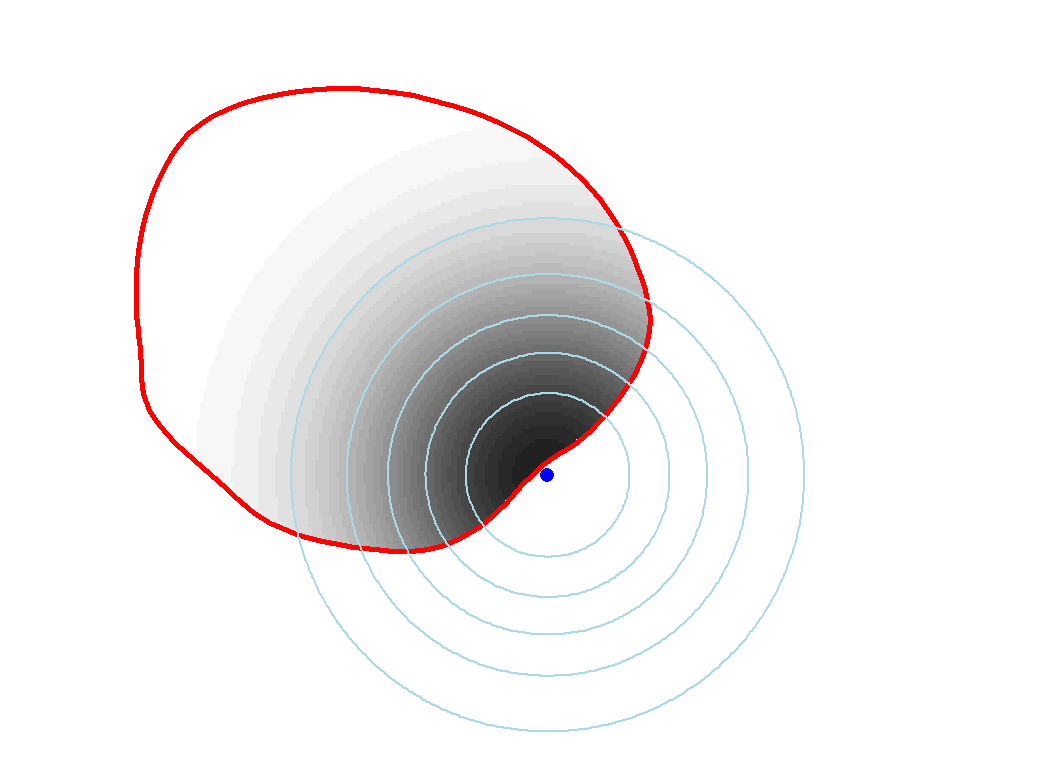
The distance-dependent detection model for point detectors is replaced for area searches by an overlap model. The hazard of detection of an individual within an irregular searched area is modelled as a function of the quantitative overlap between its home range¹ (assumed circular) and the area searched (Fig. 4.1).

Figure 4.1: Hazard of detection for an animal centered at the blue dot on an irregular searched polygon (red outline). The cumulative hazard is modelled by the quantitative overlap (grey shading) between a radially symmetrical probability density (circular contours) and the searched area.

We use \lambda_0 for the expected number of detections (detected cues) of an animal whose home range lies completely within the area \kappa, and h(\mathbf u|\mathbf x) for the probability density of activity at point \mathbf u for an animal centred at \mathbf x (i.e. \int_{R^2} h(\mathbf u|\mathbf x) \, d \mathbf u = 1). Then the expected number of detected cues from an individual on occasion s in polygon k is

h_{sk}(\mathbf x; \theta) = \lambda_0 \int_{\kappa_k} h(\mathbf u|\mathbf x; \theta^-) \, du, \tag{4.1}

where \theta = (\lambda_0, \theta^-) is the vector of detection parameters and \kappa_k refers to the k-th polygon. The probability of at least one detected cue is p_{sk}(\mathbf x) = 1 - \exp[-h_{sk}(\mathbf x)] as before. The detector-level probabilities conditional on AC location \mathbf x follow directly from Table 3.3 (repeated in Table 4.1).

Table 4.1: Detector-level probabilities for area-search detector types

Detector type	\mathrm{Pr}(\omega_{isk} | \mathbf x)	p_\cdot(\mathbf x)
Count polygon
Poisson	\{h_{sk} (\mathbf x)^{\omega_{isk}} \exp [-h_{sk}(\mathbf x)]\} / \omega_{isk}!	1 - \exp [- \sum_s \sum_k h_{sk}(\mathbf x)]
Binomial	\binom{B_s}{\omega_{isk}} p_{sk}(\mathbf x)^{\omega_{isk}} [1-p_{sk}(\mathbf x)]^{(B_s-\omega_{isk})}	1 - \prod_s\prod_k [1 - p_{sk} (\mathbf x)]^{B_s}
Exclusive polygon1	\{1 - \exp [-H_s(\mathbf x)]\}\frac{h_{sk}(\mathbf x)}{H_s(\mathbf x)}	1 - \exp[ -\sum_s H_s(\mathbf x)]

1. H_s = \sum_k h_{sk}(\mathbf x) is the hazard summed over areas. If a single polygon is searched then h_{sk}(\mathbf x) = H_s(\mathbf x), simplifying the expression for \mathrm{Pr}(\omega_{isk} | \mathbf x).

4.1.2 Location within searched polygon

The only data we have considered to this point are the occasion- and detector-specific binary or integer values \omega_{isk} that record detections at the level of polygons. Each spatial detection history \omega_i also includes within-polygon locations. These provide important information on detection scale \sigma and spatial variation in density \phi, and we need to include them in the likelihood.

Figure 4.2: Cues of one animal (yellow) within a searched polygon (red outline).

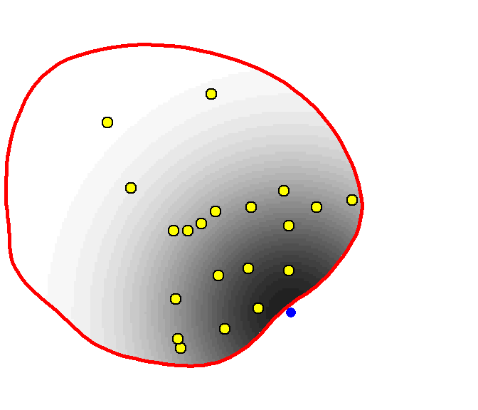
For each individual i there are \omega_{isk} locations of detected cues on occasion s at detector k. We use \mathbf Y_{isk} for the collection and \mathbf y_{iskj} (j = 1,...,\omega_{isk}) for each separate location. Then \mathrm{Pr}(\mathbf Y_{isk} | \mathbf x, \theta^-) \propto \prod_{j=1}^{\omega_{isk}} \frac{h(\mathbf y_{iskj} | \mathbf x; \theta^-)}{\int_{\kappa_k} h(\mathbf u|\mathbf x; \theta^-) \, du}. \tag{4.2}

4.1.3 Likelihood

The likelihood component associated with \omega_i, conditional on \mathbf x, is a product of the probability of observing \omega_{isk} cues, and the probability of the within-polygon locations: \mathrm{Pr}(\omega_i | \omega_i > 0, \mathbf x; \phi, \theta) \propto \frac{1}{p_\cdot(\mathbf x; \theta)} \prod_s \prod_k \mathrm{Pr}(\omega_{isk} | \mathbf x; \theta) \, \mathrm{Pr}(\mathbf Y_{isk} | \mathbf x, \theta^-). Inserted in Eq. 3.3, along with f(\mathbf x | \omega_i>0; \phi, \theta) from Eq. 3.5, this provides the likelihood component \mathrm{Pr} (\Omega | n, \phi, \theta) of Eq. 3.1.

4.2 Transect search

Transect detectors are the linear equivalent of polygons. Cues may be observed only along the searched zero-width transect. Transect detectors, like polygon detectors, may be independent or exclusive. See Appendix D for more.

Efford, M. G. (2011). Estimation of population density by spatially explicit capture-recapture analysis of data from area searches. Ecology, 92, 2202–2207.

Kendeigh, S. C. (1944). Measurement of bird populations. Ecological Monographs, 14, 67–106. https://doi.org/10.2307/1961632

Royle, J. A., Chandler, R. B., Sollmann, R., & Gardner, B. (2014). Spatial capture-recapture. Academic Press.

Royle, J. A., & Young, K. V. (2008). A hierarchical model for spatial capture-recapture data. Ecology, 89, 2281–2289.

---

1. ‘Home range’ is used here loosely - a more nuanced explanation would distinguish between the stationary distribution of activity (the home-range utilisation distribution) and the spatial distribution of cues (opportunities for detection) generated by an individual.