In addition to the variation that can be attributed to covariates (e.g., sex) or specific effects (occasion, learned responses etc.) there may be variation in detection parameters among individuals that is unrelated to known predictors. This goes by the name ‘individual heterogeneity’. Unmodelled individual heterogeneity can be a major source of bias in non-spatial capture–recapture estimates of population size (Otis et al., 1978).
It has long been recognised that SECR removes one major source of individual heterogeneity by modelling differential access to detectors. However, each detection parameter (g_0, \lambda_0, \sigma) is potentially heterogeneous and a source of bias in SECR estimates of density, as we saw in Chapter 6.
Individual heterogeneity may be addressed by treating the parameter as a random effect. This entails integrating the likelihood over the hypothesized distribution of the parameter. Results are unavoidably dependent on the choice of distribution. The distribution may be continuous or discrete. Finite mixture models with a small number of latent classes (2 or 3) are a form of random effect that is particularly easy to implement (Pledger, 2000).
Continuous random effects are usually assumed to follow a normal distribution on the link scale. There are numerical methods for efficient integration of normal random effects, but these have not been implemented in secr. Despite its attractive smoothness, a normal distribution lacks some of the statistical flexibility of finite mixtures. For example, the normal distribution has fixed skewness, whereas a 2-class finite mixture allows varying skewness. The likelihood for finite mixtures is described separately.
Interpreting latent classes
It’s worth mentioning a perennial issue of interpretation: Do the latent classes in a finite mixture model have biological reality? The answer is ‘Probably not’ (although the hybrid model blurs this issue). Fitting a finite mixture model does not require or imply that there is a matching structure in the population (discrete types of animal). A mixture model is merely a convenient way to capture heterogeneity.
Mixture models are prone to fitting problems caused by multimodality of the likelihood. Some comments are offered below, but a fuller investigation is needed.
In a finite mixture model no individual is known with certainty to belong to a particular class, although membership probability may be assigned retrospectively from the fitted model. A hybrid model may incorporate the known class membership of some or all individuals, as we described in Chapter 5.
15.1 Finite mixture models in secr
secr allows 2- or 3-class finite mixture models for any ‘real’ detection parameter (e.g., g0, lambda0 or sigma of a halfnormal detection function). Consider a simple example in which we specify a 2-class mixture by adding the predictor ‘h2’ to the model formula:
Continuing with the snowshoe hares:
fit.h2<-secr.fit(hareCH6, model =lambda0~h2, detectfn ='HEX', buffer =250, trace =FALSE)coef(fit.h2)
secr.fit has expanded the model to include an extra ‘real’ parameter ‘pmix’, for the proportions in the respective latent classes. You could specify this yourself as part of the ‘model’ argument, but secr.fit knows to add it. The link function for ‘pmix’ defaults to ‘mlogit’ (after the mlogit link in MARK), and any attempt to change the link is ignored.
There are two extra ‘beta’ parameters: lambda0.h22, which is the difference in lambda0 between the classes on the link (logit) scale, and pmix.h22, which is the proportion in the second class, also on the logit scale. Fitted (real) parameter values are reported separately for each mixture class (h2 = 1 and h2 = 2). An important point is that exactly the same estimate of total density is reported for both mixture classes; the actual abundance of each class is D \times pmix.
Warning
When more than one real parameter is modelled as a mixture, there is an ambiguity: is the population split once into latent classes common to all real parameters, or is the population split separately for each real parameter? The second option would require a distinct level of the mixing parameter for each real parameter. secr implements only the ‘common classes’ option, which saves one parameter.
We now shift to a more interesting example based on the Coulombe’s house mouse Mus musculus dataset (Otis et al., 1978).
Although the best mixture model fits substantially better than the null model (\DeltaAIC = 33.3), there is only a 2.6% difference in \hat D. More complex models are allowed. For example, one might, somewhat outlandishly, fit a learned response to capture that differs between two latent classes, while also allowing sigma to differ between classes:
model.h2xbh2s<-secr.fit(morning, model =list(lambda0~h2*bk, sigma~h2), buffer =25, detectfn ='HEX')
15.1.1 Number of classes
The theory of finite mixture models in capture–recapture (Pledger, 2000) allows an indefinite number of classes – 2, 3 or perhaps more. Programmatically, the extension to more classes is obvious (e.g., h3 for a 3-class mixture). The appropriate number of latent classes may be determined by comparing AIC for the fitted models.
Looking on the bright side, it is unlikely that you will ever have enough data to support more than 2 classes. For the data in the example above, the 2-class and 3-class models have identical log likelihood to 4 decimal places, while the latter requires 2 extra parameters to be estimated (this is to be expected as the data were simulated from a null model with no heterogeneity).
15.1.2 Label switching
It is a quirk of mixture models that the labeling of the latent classes is arbitrary: the first class in one fit may become the second class in another. This is the phenomenon of ‘label switching’ (Stephens, 2000).
For example, in the house mouse model ‘h2.lambda0’ the first class is initially dominant, but we can switch that by choosing different starting values for the maximization:
Class-specific estimates of the detection parameter (here lambda0) are reversed, but estimates of other parameters are unaffected.
15.1.3 Multimodality
The likelihood of a finite mixture model may have multiple modes (Brooks et al., 1997; Pledger, 2000). The risk is ever-present that the numerical maximization algorithm will get stuck on a local peak, and in this case the estimates are simply wrong. Slight differences in starting values or numerical method may result in wildly different answers.
The problem has not been explored fully for SECR models, and care is needed. Pledger (2000) recommended fitting a model with more classes as a check in the non-spatial case, but this is not proven to work with SECR models. It is desirable to try different starting values. This can be done simply using another model fit. For example:
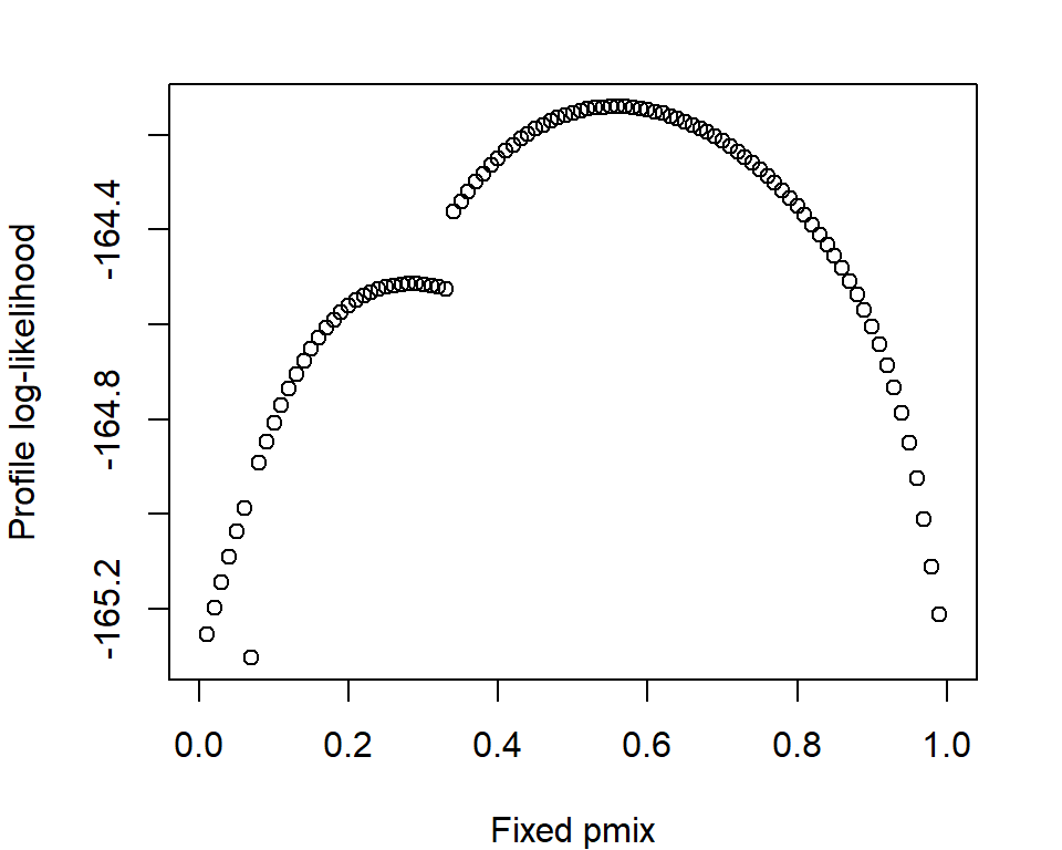
A more time consuming, but illuminating, check on a 2-class model is to plot the profile log likelihood for a range of mixture proportions (Brooks et al., 1997). We can use the function pmixprofileLL in secr to calculate these profile likelihoods. This requires a maximization step for each value of ‘pmix’; multiple cores may be used in parallel to speed up the computation. pmixprofileLL expects the user to identify the coefficient or ‘beta parameter’ corresponding to ‘pmix’ (argument ‘pmi’):
code for profile likelihood plot
pmvals<-seq(0.01,0.99,0.01)# use a coarse mask to make it fastermask<-make.mask(traps(ovenCH[[1]]), nx =32, buffer =200, type ="trapbuffer")profileLL<-pmixProfileLL(ovenCH[[1]], model =list(lambda0~h2, sigma~h2), pmi =5, detectfn ='HEX', CL =TRUE, pmvals =pmvals, mask =mask, trace =FALSE)par(mar =c(4,4,2,2))plot(pmvals, profileLL, xlim =c(0,1), xlab ='Fixed pmix', ylab ='Profile log-likelihood')
Figure 15.1: Profile log-likelihood for mixing proportion between 0.01 and 0.99 in a 2-class finite mixture model for ovenbird data from 2005
Multimodality is likely to show up as multiple rounded peaks in the profile likelihood. Label switching may cause some ghost reflections about pmix = 0.5 that can be ignored. If multimodality is found one should accept only estimates for which the maximized likelihood matches that from the highest peak. In the ovenbird example, the maximized log likelihood of the fitted h2 model was -163.8 and the estimated mixing proportion was 0.51, so the correct maximum was found.
Maximization algorithms (argument ‘method’ of secr.fit) differ in their tendency to settle on local maxima; ‘Nelder-Mead’ is probably better than the default ‘Newton-Raphson’. Simulated annealing is sometimes advocated, but it is slow and has not been tried with SECR models.
15.2 Mitigating factors
Heterogeneity may be demonstrably present yet have little effect on density estimates. Bias in density is a non-linear function of the coefficient of variation of a_i(\theta). For CV <20\% the bias is likely to be negligible (Efford & Mowat, 2014).
Individual variation in \lambda_0 and \sigma may be inversely correlated and therefore compensatory, reducing bias in \hat D(Efford & Mowat, 2014). Bias is a function of heterogeneity in the effective sampling areaa(\theta) which may vary less than each of the components \lambda_0 and \sigma.
It can be illuminating to re-parameterize the detection model.
15.3 Hybrid ‘hcov’ model
The hybrid mixture model accepts a 2-level categorical (factor) individual covariate for class membership that may be missing (NA) for any fraction of animals. The name of the covariate to use is specified as argument ‘hcov’ in secr.fit. If the covariate is missing for all individuals then a full 2-class finite mixture model will be fitted (i.e. mixture as a random effect). Otherwise, the random effect applies only to the animals of unknown class; others are modelled with detection parameter values appropriate to their known class. If class is known for all individuals the model is equivalent to a covariate (CL = TRUE) or grouped (CL = FALSE) model. When many or all animals are of known class the mixing parameter may be treated as an estimate of population proportions (probability a randomly selected individual belongs to class u). This is obviously useful for estimating sex ratio free of detection bias. See the hcov help page (?hcov) for implementation details, and here for the theory.
The house mouse dataset includes an individual covariate ‘sex’ with 81 females, 78 males and one unknown.
Brooks, S. P., Morgan, B. J. T., Ridout, M. S., & Pack, S. E. (1997). Finite mixture models for proportions. Biometrics, 53(3), 1097. https://doi.org/10.2307/2533567
Efford, M. G., & Mowat, G. (2014). Compensatory heterogeneity in spatially explicit capture-recapture data. Ecology, 95, 1341–1348.
Otis, D. L., Burnham, K. P., White, G. C., & Anderson, D. R. (1978). Statistical inference from capture data on closed animal populations. Wildlife Monographs, 62.
Pledger, S. (2000). Unified maximum likelihood estimates for closed capture-recapture models using mixtures. Biometrics, 56, 434–442.
Stephens, M. (2000). Dealing with label switching in mixture models. Journal of the Royal Statistical Society Series B, 62, 795–809.