Appendix C — Spatial data

These notes explain how secr uses spatial data. Spatial data are used to

locate detectors (read.traps, read.capthist)
map the extent of habitat near detectors (make.mask)
attach covariates to traps or mask objects (addCovariates)
delimit regions of interest (region.N and other functions)

Some spatial results may be exported, particularly the raster density surfaces generated by predictDsurface from a fitted model.

Internally, secr uses a very simple concept of space. The locations of detectors (traps), the potential locations of activity centres (habitat mask) and the simulated locations of individuals (popn) are described by Cartesian (x-y) coordinates assumed to be in metres. Distances are Euclidean unless specifically modelled as non-Euclidean (Appendix F). Only relative positions matter for the calculations, so the origin of the coordinates is arbitrary. The map projection (‘coordinate reference system’ or CRS) is not recorded.

Most spatial computations in secr (distances, areas, overlay etc.) use internal R and C++ code. Polygon and transect detectors are represented as dataframes in which each row gives the x- and y-coordinates of a vertex and topology is ignored (holes are not allowed).

The simple approach works fine within limits (discussed later), but issues arise when secr

exchanges spatial data (regions, covariates or predicted density) with other software, or
uses functions from R spatial packages, especially sf and spsurvey.

C.1 Spatial data in R

To use spatial data or functions from external sources in secr it helps to know a little about the expanding spatial ecosystem in R.

C.1.1 R packages for spatial data

Several widely used packages define classes and methods for spatial data (‘Used by’ in the following table is the number of CRAN packages from crandep::get_dep on 2025-02-10).

Package	Scope	Year	Used by	Citation	Relevant S4 classes
sp	vector	2005–	465	Pebesma & Bivand (2005)	SpatialPolygons, SpatialPolygonsDataFrame, SpatialGridDataFrame, SpatialLinesDataFrame
raster	raster	2010–	339	Hijmans (2023a)	RasterLayer
sf	vector	2016–	936	Pebesma (2018)	sfg, sfc, sf
stars	both	2018–	79	Edzer & Bivand (2023)	stars
terra	both	2020–	398	Hijmans (2023b)	SpatVector, SpatRaster

The reader should already understand the distinction between vector and raster spatial data. There are many resources for learning about spatial analysis in R that may be found by web search on, for example ‘R spatial data’. The introduction by Claudia Engel covers both sp and sf.

The capability of sp is being replaced by sf and raster is being replaced by terra. The more recent packages tend to be faster. sf implements the ‘simple features’ standard.

C.1.2 Geographic vs projected coordinates

QGIS has an excellent introduction to coordinate reference systems (CRS) for GIS. Coordinate reference systems may be specified in many ways; the most simple is the 4- or 5-digit EPSG code (search for EPSG on the web).

Geographic coordinates (EPSG 4326, ignoring some details) specify a location on the earth’s surface by its latitude and longitude. This is the standard in Google Earth and Geographic Positioning Systems (GPS).

C.2 Spatial data in secr

C.2.1 Input of detector locations

secr uses relative Cartesian coordinates. Detector coordinates from GPS should therefore be projected from geographic coordinates before input to secr. Most of the R spatial packages include projection functions. Here is a simple example using st_transform from the sf package:

library(sf)

Linking to GEOS 3.11.2, GDAL 3.7.2, PROJ 9.3.0; sf_use_s2() is TRUE

# unprojected (geographic) coordinates (decimal degrees) 
# longitude before latitude
df <- data.frame(x = c(174.9713, 174.9724, 174.9738), 
                 y = c(-41.3469, -41.3475, -41.3466))
# construct sf object
latlon <- st_as_sf(df, coords = 1:2)
# specify initial CRS: WGS84 lat-lon
st_crs(latlon) <- 4326  
# project to Cartesian coordinate system, units metres
# EPSG:27200 is the old (pre-2001) NZMG
trps <- st_transform(latlon, crs = 27200) 
# print
st_coordinates(latlon)

          X       Y
[1,] 174.97 -41.347
[2,] 174.97 -41.347
[3,] 174.97 -41.347

st_coordinates(trps)

           X       Y
[1,] 2674948 5982573
[2,] 2675038 5982504
[3,] 2675157 5982602

C.2.2 Adding spatial covariates to a traps or mask object

SECR models may include covariates for each detector (e.g., trap or searched polygon) in the detection model (parameters g_0, \lambda_0, \sigma etc.) and for each point on the discretized habitat mask in the density model (parameter D).

Covariates measured at detector locations may be included in the text files read by read.traps or read.capthist.

Covariates measured at each point on a habitat mask may be included in a file or data.frame input to read.mask, but this is an uncommon way to establish mask covariates. More commonly, a habitat mask is built using make.mask and initially has no covariates,

The function addCovariates is a convenient way to attach covariates to a traps or mask object post hoc. The function extracts covariate values from the ‘spatialdata’ argument by a spatial query for each point on a mask. Options are

spatialdata	Notes
character	name of ESRI shapefile, excluding ‘.shp’
sp::SpatialPolygonsDataFrame
sp::SpatialGridDataFrame
raster::RasterLayer
secr::mask	covariates of nearest point
secr::traps	covariates of nearest point
terra::SpatRaster	new in 4.5.3
sf::sf	new in 4.5.3

Data sources should use the coordinate reference system of the target detectors and mask (see previous section).

C.2.3 Functions with ‘poly’ or ‘region’ spatial argument

Several secr functions use spatial data to define a region of interest (i.e. one or more polygons). All such polygons may be defined as

2-column matrix or data.frame of x- and y-coordinates
SpatialPolygons or SpatialPolygonsDataFrame S4 classes from package sp
SpatRaster S4 class from package terra
sf or sfc S4 classes from package sf (POLYGON or MULTIPOLYGON geometries)

Data in these formats are converted to an object of class sfc by the documented internal function boundarytoSF. The S4 classes allow complex regions with multiple polygons (islands), possibly containing ‘holes’ (lakes).

This applies to the following functions and arguments:

secr function	Argument
bufferContour	poly
deleteMaskPoints	poly
esaPlot	poly
make.mask	poly
make.systematic	region
mask.check	poly
pdotContour	poly
PG	poly
pointsInPolygon	poly*
region.N	region*
sim.popn	poly
subset.popn	poly
trap.builder	region
trap.builder	exclude

* pointsInPolygon and region.N also accept a habitat mask.

C.2.4 GIS functionality imported from other R packages

Some specialised spatial operations are out-sourced by secr:

secr function	Operation	Other-package function	Reference
randomHabitat	simulated habitat	raster::adjacent	Hijmans (2023a)
		raster::clump
nedist	non-Euclidean distances	gdistance::transition	van Etten (2023)
		gdistance::geoCorrection
		gdistance::costDistance
discretize	cell overlap with polygon(s)	sf::st_intersection	Pebesma (2018)
		sf::st_area
polyarea	area of polygon(s)	sf::st_area
make.mask	polybuffer mask type	sf::st_buffer
rbind.capthist	merge polygon detectors	sf::st_union
trap.builder	SRS sample	sf::st_sample
trap.builder	GRTS sample (spsurvey >= 5.3.0)	spsurvey::grts	Dumelle et al. (2024)

C.2.5 Exporting raster data for use in other packages

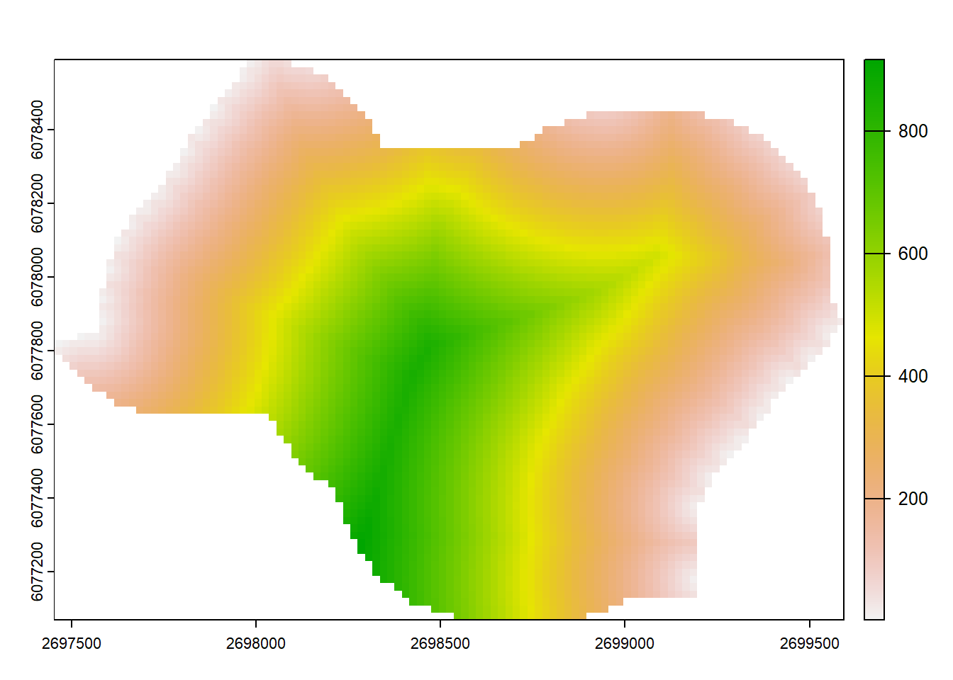
A mask or predicted density surface (Dsurface) generated in secr may be used or plotted as a raster layer in another R package. secr provides rast and raster methods for secr mask and Dsurface objects, based on the respective generic functions exported by terra and raster. These return SpatRaster and RasterLayer objects respectively. For example,

library(secr)
summary(possummask)

Object class      mask 
Mask type         trapbuffer 
Number of points  5120 
Spacing m         20 
Cell area ha      0.04 
Total area ha     204.8 
x-range m         2697463 2699583 
y-range m         6077080 6078580 
Bounding box      
        x       y
1 2697453 6077070
2 2699593 6077070
4 2699593 6078590
3 2697453 6078590

Summary of covariates 
   d.to.shore    
 Min.   :  2.24  
 1st Qu.:200.11  
 Median :370.80  
 Mean   :389.24  
 3rd Qu.:560.82  
 Max.   :916.69

# make SpatRaster object from mask covariate
r <- rast(possummask, covariate = 'd.to.shore')
print(r)

class       : SpatRaster 
dimensions  : 76, 107, 1  (nrow, ncol, nlyr)
resolution  : 20, 20  (x, y)
extent      : 2697453, 2699593, 6077070, 6078590  (xmin, xmax, ymin, ymax)
coord. ref. :  
source(s)   : memory
name        :      tmp 
min value   :   2.2361 
max value   : 916.6924

terra::plot(r)

C.3 Limits of the Cartesian model in secr

C.3.1 Distances computed in large studies

Distances on the curved surface of the earth are not well represented by straight-line Euclidean distances when the study area is very large, as happens with large carnivores such as grizzly bears and wolverines. That has led some authors to use more rigorous (great-circle) distances. This is not possible in secr because there is no record of the projected coordinate reference system used for the detectors and habitat mask.