# Session ID Occasion Detector sex
1 1 3 H4 f
1 10 2 A1 f
1 11 4 D2 m
1 12 1 B3 f
.
.
2 1 2 A8 m
2 1 4 A8 m
2 10 4 A5 f
2 11 2 A6 f
.
.
3 1 4 D6 m
3 10 3 A1 m
3 11 2 G3 m
3 11 4 H6 m
.
.14 Multiple sessions
A ‘session’ in secr is a block of sampling that may be treated as independent from all other sessions. For example, sessions may correspond to trapping grids that are far enough apart that they sample non-overlapping sets of animals. Multi-session data and models combine data from several sessions. Sometimes this is merely a convenience, but it also enables the fitting of models with parameter values that apply across sessions – data are then effectively pooled with respect to those parameters.
Multi-session data are referred to as ‘stacked’ data in other contexts (Kéry & Royle, 2020, pp. 67, 76).
Dealing with multiple sessions adds another layer of complexity, and raises some entirely new issues. This chapter tries for a coherent view of multi-session analyses, covering material that is otherwise scattered.
14.1 Input
A multi-session capthist object is essentially an R list of single-session capthist objects. We assume the functions read.capthist or make.capthist will be used for data input (simulated data are considered separately later on).
14.1.1 Detections
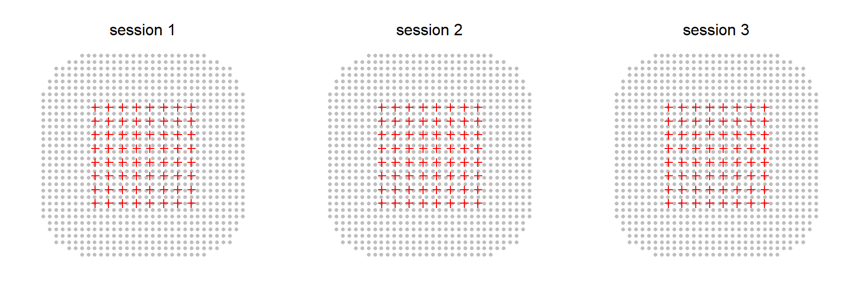
Entering session-specific detections is simple because all detection data are placed in one file or dataframe. Each session uses a character-valued code (the session identifier) in the first column. For demonstration let’s assume you have a file ‘msCHcapt.txt’ with data for 3 sessions, each sampled on 4 occasions.
(clipped lines are indicated by ‘. .’).
Given a trap layout file ‘msCHtrap.txt’ with the coordinates of the detector sites (A1, A2 etc.), the following call of read.capthist will construct a single-session capthist object for each unique code value and combine these in a multi-session capthist:
msCH <- read.capthist('data/msCHcapt.txt', 'data/msCHtrap.txt', covnames = 'sex')No errors found :-)Use the summary method or str(msCH) to examine msCH. Session-by-session output from summary can be excessive; the ‘terse’ option gives a more compact summary across sessions (columns).
summary(msCH, terse = TRUE) 1 2 3
Occasions 4 4 4
Detections 52 55 42
Animals 31 31 27
Detectors 64 64 64Sessions are ordered in msCH according to their identifiers (‘1’ before ‘2’, ‘Albert’ before ‘Beatrice’ etc.). The order becomes important for matching with session-specific trap layouts and masks, as we see later. The vector of session names (identifiers) may be retrieved with session(msCH) or names(msCH).
14.1.2 Empty sessions
It is possible for there to be no detections in some sessions (but not all!). To create a session with no detections, include a dummy row with the value of the noncapt argument as the animal identifier; the default noncapt value is ‘NONE’. The dummy row should have occasion number equal to the number of occasions and some nonsense value (e.g. 0) in each of the other fields (trapID etc.).
Including individual covariates as additional columns seems to cause trouble in the present version of secr if some sessions are empty, and should be avoided. We drop them from the example file ‘msCHcapt2.txt’:
# Session ID Occasion Detector
1 19 2 A1
1 28 2 A5
1 37 2 A6
.
.
3 25 1 A5
3 16 4 A5
3 21 3 A6
3 6 1 A7
.
.
4 NONE 4 0
Then,
msCH2 <- read.capthist('data/msCHcapt2.txt', 'data/msCHtrap.txt')Session 4
No live releasessummary(msCH2, terse = TRUE) 1 2 3 4
Occasions 4 4 4 4
Detections 63 52 50 0
Animals 39 29 31 0
Detectors 64 64 64 64Empty sessions trigger an error in verify.capthist; to fit a model suppress verification (e.g., secr.fit(msCH2, verify = FALSE)).
If the first session is empty then either direct the autoini option to a later session with e.g., details = list(autoini = 2) or provide initial values manually in the start argument.
14.1.3 Detector layouts
All sessions may share the same detector layout. Then the ‘trapfile’ argument of read.capthist is a single name, as in the example above. The trap layout is repeated as an attribute of each component (single-session) capthist.
Alternatively, each session may have its own detector layout. Unlike the detection data, each session-specific layout is specified in a separate input file or traps object. For read.capthist the ‘trapfile’ argument is then a vector of file names, one for each session. For make.capthist, the ‘traps’ argument may be a list of traps objects, one per session. The first trap layout is used for the first session, the second for the second session, etc.
14.2 Manipulation
The standard extraction and manipulation functions of secr (summary, verify, covariates, subset, reduce etc.) mostly allow for multi-session input, applying the manipulation to each component session in turn. The function ms returns TRUE if its argument is a multi-session object and FALSE otherwise.
Plotting a multi-session capthist object (e.g., plot(msCH)) will create one new plot for each session unless you specify add = TRUE.
Methods that extract attributes from multi-session capthist object will generally return a list in which each component is the result from one session. Thus for the ovenbird mistnetting data traps(ovenCH) extracts a list of 5 traps objects, one for each annual session 2005–2009.
The subset method for capthist objects has a ‘sessions’ argument for selecting particular session(s) of a multi-session object.
| Function | Purpose | Input | Output |
|---|---|---|---|
join |
collapse sessions | multi-session CH | single-session CH |
MS.capthist |
build multi-session CH | several single-session CH | multi-session CH |
split |
subdivide CH | single-session CH | multi-session CH |
| multi-session CH | several multi-session CH |
The split method for capthist objects (?split.capthist) may be used to break a single-session capthist object into a multi-session object, segregating detections by some attribute of the individuals, or by occasion or detector groupings. Also, from secr 5.0.1, the split method may be used to group sessions in a multi-session capthist.
14.3 Fitting
Given multi-session capthist input, secr.fit automatically fits a multi-session model by maximizing the product of session-specific likelihoods (Efford et al., 2009). For fitting a model separately to each session see the later section on Faster fitting….
14.3.1 Habitat masks
The default mechanism for constructing a habitat mask in secr.fit is to buffer around the trap layout. This extends to multi-session data; buffering is applied to each trap layout in turn.
Override the default buffering mechanism by specifying the ‘mask’ argument of secr.fit. This is necessary if you want to –
- reduce or increase mask spacing (pixel size; default 1/64 x-range)
- clip the mask to exclude non-habitat
- include mask covariates (predictors of local density)
- define non-Euclidean distances (Appendix F)
- specify a rectangular mask (type = “traprect” vs type = “trapbuffer”)
For any of these you are likely to use the make.mask function (the manual alternative is usually too painful to contemplate). If make.mask is provided with a list of traps objects as its ‘traps’ argument then the result is a list of mask objects - effectively, a multi-session mask.
If addCovariates receives a list of masks and a single spatial data source then it will add the requested covariate(s) to each mask and return a new list of masks. The single spatial data source is expected to span all the regions; mask points that are not covered receive NA covariate values. As an alternative to a single spatial data source, the spatialdata argument may be a list of spatial data sources, one per mask, in the order of the sessions in the corresponding capthist object.
To eliminate any doubt about the matching of session-specific masks to session-specific detector arrays it is always worth plotting one over the other. We don’t have an interesting example, but
14.3.2 Session models
The default in secr.fit is to treat all parameters as constant across sessions. For detection functions parameterized in terms of cumulative hazard (e.g., ‘HHN’ or ‘HEX’) this is equivalent to model = list(D ~ 1, lambda0 ~ 1, sigma ~ 1). Two automatic predictors are provided specifically for multi-session models: ‘session’ and ‘Session’.
14.3.2.1 Session-stratified estimates
A model with lowercase ‘session’ fits a distinct value of the parameter (D, g0, lambda0, sigma) for each level of factor(session(msCH)).
14.3.2.2 Session covariates
Other variation among sessions may be modelled with session-specific covariates. These are provided to secr.fit on-the-fly in the argument ‘sessioncov’ (they cannot be embedded in the capthist object like detector or individual covariates). The value for ‘sessioncov’ should be a dataframe with one row per session. Each column is a potential predictor in a model formula; other columns are ignored.
Session covariates are extremely flexible. The linear trend of the ‘Session’ predictor may be emulated by defining a covariate sessnum = 0:(R-1) where R is the number of sessions. Sessions of different types may be distinguished by a factor-valued covariate. Supposing for the ovenbird dataset we wished to distinguish years 2005 and 2006 from 2007, 2008 and 2009, we could use earlylate = factor(c('early','early','late','late','late')). Quantitative habitat attributes might also be coded as session covariates.
14.3.2.3 Trend across sessions
secr is primarily for estimating closed population density (density at one point in time), but multi-session data may also be modelled to describe population trend over time. A trend model for density may be interesting if the sessions fall in some natural sequence, such as a series of annual samples (as in the ovenbird dataset ovenCH). A model with initial uppercase ‘Session’ fits a trend across sessions using the session number as the predictor. The fitted trend is linear on the link scale; using the default link function for density (‘log’) this corresponds to exponential growth or decline if samples are equally spaced in time.
The pre-fitted model ovenbird.model.D provides an example. The coefficient ‘D.Session’ is the rate of change in log(D):
coef(ovenbird.model.D) beta SE.beta lcl ucl
D 0.031711 0.191460 -0.34354 0.406966
D.Session -0.063859 0.070151 -0.20135 0.073635
g0 -3.561933 0.150623 -3.85715 -3.266718
sigma 4.364111 0.081149 4.20506 4.523159The overall finite rate of increase (equivalent to Pradel’s lambda) is given by
beta <- coef(ovenbird.model.D)['D.Session','beta']
sebeta <- coef(ovenbird.model.D)['D.Session','SE.beta']
exp(beta)
[1] 0.93814Confidence intervals may also be back-transformed with exp. To back-transform the SE use the delta-method approximation exp(beta) * sqrt(exp(sebeta^2)-1) = 0.06589.
This is fine for a single overall lambda. However, if you are interested in successive estimates (session 1 to session 2, session 2 to session 3 etc.) the solution is slightly more complicated. Here we describe a simple option using ‘backward difference’ coding of the levels of the factor session, specified with the details argument ‘contrasts’. This coding is provided by the function contr.sdif in the MASS package (e.g., Venables and Ripley 1999 Section 6.2).
fit <- secr.fit(ovenCH, model = D~session, buffer = 300, trace = FALSE,
    details = list(contrasts = list(session = MASS::contr.sdif)))
coef(fit)
A more sophisticated version is provided in Appendix J.
14.4 Simulation
Back at the start of this document we used sim.capthist to generate msCH, a simple multi-session capthist. Here we look at various extensions. Generating SECR data is a 2-stage process. The first stage simulates the locations of animals to create an object of class ‘popn’; the second stage generates samples from that population according to a particular sampling regime (detector array, number of occasions etc.).
14.4.1 Simulating multi-session populations
By default sim.capthist uses sim.popn to generate a new population independently for each session. Centres are placed within a rectangular region obtained by buffering around a ‘core’ (the traps object passed to sim.capthist).
The session-specific populations may also be prepared in advance as a list of ‘popn’ objects (use nsessions > 1 in sim.popn). This allows greater control. In particular, the population density may be varied among sessions by making argument D a vector of session-specific densities. Other arguments of sim.popn do not yet accept multi-session input – it might be useful for ‘core’ to accept a list of traps objects (or a list of mask objects if model2D = “IHP”).
We can also put aside the basic assumption of independence among sessions and simulate a single population open to births, deaths and movement between sessions. This does not correspond to any model that can be fitted in secr, but it allows the effects of non-independence to be examined. See ?turnover for further explanation.
14.4.2 Multi-session sampling
A multi-session population prepared in advance is passed as the popn argument of sim.capthist, replacing the usual list (D, buffer etc.).
The argument ‘traps’ may be a list of length equal to nsessions. Each component potentially differs not just in detector locations, but also with respect to detector type (‘detector’) and resighting regime (‘markocc’). The argument ‘noccasions’ may also be a vector with a different number of occasions in each session.
14.5 Problems
There are problems specific to multi-session data.
14.5.1 Failure of autoini
Numerical maximization of the likelihood requires a starting set of parameter values. This is either computed internally with the function autoini or provided by the user. Given multi-session data, the default procedure is for secr.fit to apply autoini to the first session only. If the data for that session are inadequate or result in parameter estimates that are extreme with respect to the remaining sessions then model fitting may abort. One solution is to provide start values manually, but that can be laborious. A quick fix is often to switch the session used to compute starting values by changing the details option ‘autoini’. For example
fit0 <- secr.fit(ovenCH, mask = msk, details = list(autoini = 2), trace = FALSE)A further option is to combine the session data into a single-session capthist object with details = list(autoini = "all"); the combined capthist is used only by autoini.
14.6 Speed
Fitting a multi-session model with each parameter stratified by session is unnecessarily slow. In this case no data are pooled across sessions and it is better to fit each session separately. If your data are already in a multi-session capthist object then the speedy solution is
msk <- make.mask(traps(ovenCH[[1]]), buffer = 300, nx = 25, type = 'trapbuffer')
fits <- lapply(ovenCH, secr.fit, mask = msk, trace = FALSE)
class(fits) <- 'secrlist'
predict(fits)
$`2005`
link estimate SE.estimate lcl ucl
D log 0.846489 0.3055467 0.426316 1.680780
g0 logit 0.023247 0.0082002 0.011591 0.046079
sigma log 88.124224 19.4762683 57.439449 135.201136
$`2006`
link estimate SE.estimate lcl ucl
D log 1.026929 0.2936740 0.592771 1.779071
g0 logit 0.030126 0.0092789 0.016396 0.054715
sigma log 73.020556 11.7120666 53.429792 99.794541
$`2007`
link estimate SE.estimate lcl ucl
D log 1.078170 0.2879556 0.644547 1.803516
g0 logit 0.034768 0.0093266 0.020465 0.058471
sigma log 76.079441 11.5022360 56.663445 102.148419
$`2008`
link estimate SE.estimate lcl ucl
D log 1.468095 0.488689 0.77772 2.771315
g0 logit 0.028298 0.011253 0.01289 0.060988
sigma log 52.223609 10.478510 35.38004 77.085985
$`2009`
link estimate SE.estimate lcl ucl
D log 0.531270 0.2009519 0.259448 1.087876
g0 logit 0.024442 0.0088054 0.012003 0.049129
sigma log 98.909058 22.8569244 63.253482 154.663449The first line (lapply) creates a list of ‘secr’ objects. The predict method works once we set the class attribute to ‘secrlist’ (or you could lapply(fits, predict)).
fits2 <- secr.fit(ovenCH, model=list(D~session, g0~session,
    sigma~session), mask = msk, trace = FALSE)
What if we wish to compare ths model with a less general one (i.e. with some parameter values shared across sessions)? For that we need the number of parameters, log likelihood and AIC summed across sessions:
Warning: models not compatible for AIC npar logLik AIC
15.00 -925.89 1881.78 AIC(fits2)[,3:5] npar logLik AIC
fits2 15 -925.89 1881.8AICc is not a simple sum of session-specific AICc and should be calculated manually (hint: use sapply(ovenCH, nrow) for session-specific sample sizes).
The unified model fit and separate model fits with lapply give essentially the same answers, and the latter approach is faster by a factor of 157.
Using lapply does not work if some arguments of secr.fit other than ‘capthist’ themselves differ among sessions (as when ‘mask’ is a list of session-specific masks). Then we can use either a ‘for’ loop or the slightly more demanding function mapply, with the same gain in speed.
# one mask per session
masks <- make.mask(traps(ovenCH), buffer = 300, nx = 32,
    type = 'trapbuffer')
fits3 <- list.secr.fit(ovenCH, mask = masks, constant =
    list(trace = FALSE))
14.7 Caveats
14.7.1 Independence is a strong assumption
If sessions are not truly independent then expect confidence intervals to be too short. This is especially likely when a trend model is fitted to temporal samples with incomplete population turnover between sessions. The product likelihood assumes a new realisation of the underlying population process for each session. If in actuality much of the sampled population remains the same (the same individuals in the same home ranges) then the precision of the trend coefficient will be overstated. Either an open population model is needed (e.g., openCR (Efford & Schofield, 2020)) or extra work will be needed to obtain credible confidence limits for the trend (probably some form of bootstrapping).
14.7.2 Parameters are assumed constant by default
Output from predict.secr for a multi-session model is automatically stratified by session even when the model does not include ‘session’, ‘Session’ or any session covariate as a predictor (the output simply repeats the constant estimates for each session).