10  Detection model

The detection model in SECR most commonly models the probability that an individual with a particular activity centre will be detected on a particular occasion at a particular place (detector). If the detector type allows for multiple detections (cues or visits) the model describes the number of detections rather than probability.

A bare-bones detection model is a distance-detection function (or simply ‘detection function’) with two parameters, intercept and spatial scale. There are three sources of complexity and opportunities for customisation:

• function shape (e.g., halfnormal vs negative exponential) and whether it describes the probability or hazard of detection,
• parameters may depend on other known variables, and
• parameters may be modelled as random effects to represent variation of unknown origin.

We consider the shape of detection functions in the next section. Modelling parameters as a function of other variables is addressed in the following section on linear submodels. Random effects in secr are limited to finite mixture models that we cover in the chapter on individual heterogeneity.

10.1 Distance-detection functions

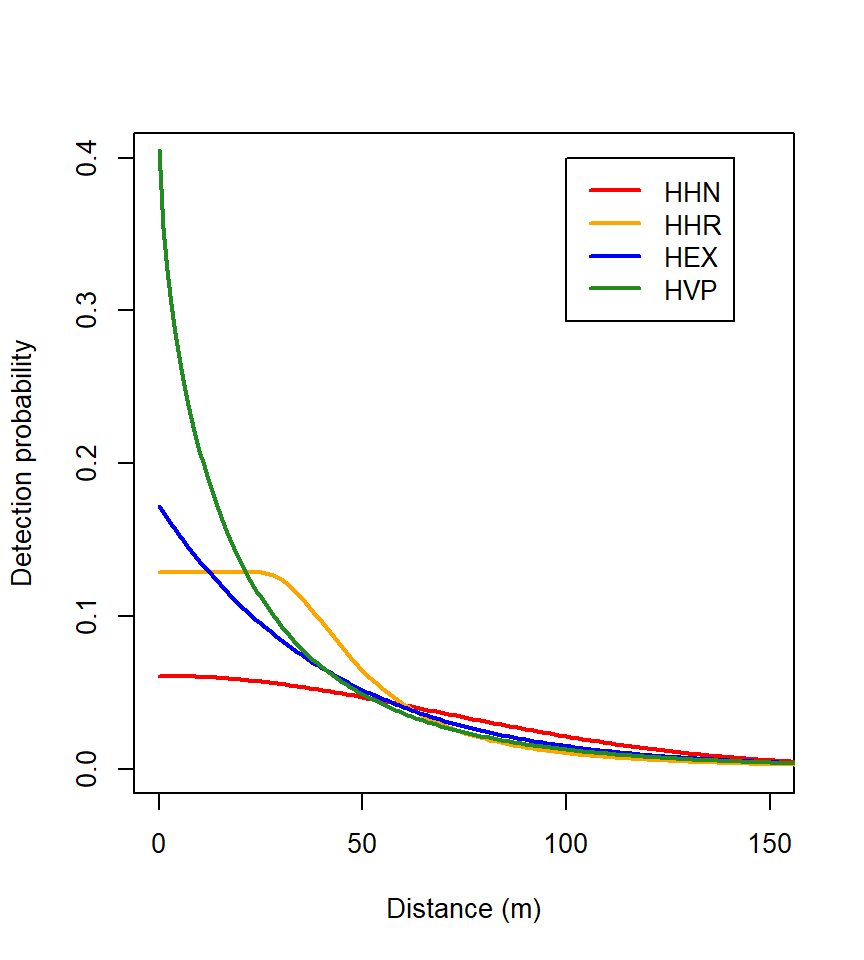
The probability of detection g(d) at a detector distance d from an activity centre may take one of the simple forms in Table 10.1. Alternatively, the probability of detection may be derived from g(d) = 1 - \exp[-\lambda(d)] where \lambda(d) is the hazard of detection, itself modelled with one of the simple parametric forms (Table 10.2)¹. Several further options are provided by secr.fit (see ? detectfn), but only ‘HN’,‘HR’, and ‘EX’ or their ‘hazard’ equivalents are commonly used.

Table 10.1: Probability detection functions.

Code	Name	Parameters	Function
HN	halfnormal	g_0, \sigma	g(d) = g_0 \exp \left(\frac{-d^2} {2\sigma^2} \right)
HR	hazard rate2	g_0, \sigma, z	g(d) = g_0 [1 - \exp\{{-(^d/_\sigma)^{-z}} \}]
EX	exponential	g_0, \sigma	g(d) = g_0 \exp \{-(^d/_\sigma) \}

Table 10.2: Hazard detection functions.

Code	Name	Parameters	Function
HHN	hazard halfnormal	\lambda_0, \sigma	\lambda(d) = \lambda_0 \exp \left(\frac{-d^2} {2\sigma^2} \right)
HHR	hazard hazard rate	\lambda_0, \sigma, z	\lambda(d) = \lambda_0 (1 - \exp \{ -(^d/_\sigma)^{-z} \})
HEX	hazard exponential	\lambda_0, \sigma	\lambda(d) = \lambda_0 \exp \{ -(^d/_\sigma) \}
HVP	hazard variable power	\lambda_0, \sigma, z	\lambda(d) = \lambda_0 \exp \{ -(^d/_\sigma)^{z} \}

The merits of focussing on the hazard³ are a little arcane. We list them here:

1. Quantities on the hazard scale are additive and more tractable for some purposes (e.g. adjusting for effort, computing expected counts).
2. For some detector types (e.g., Poisson counts) the data are integers, for which \lambda(d) has a direct interpretation as the expected count. However, \lambda(d) can always be derived from g(d) (\lambda(d) = -\log[1 - g(d)]).
3. Intuitively, there is a close proportionality between \lambda(d) and the height of an individual’s utilization pdf.

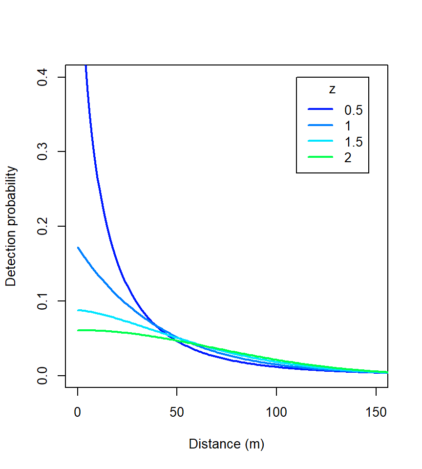
The ‘hazard variable power’ function is a 3-parameter function modelled on that of Ergon & Gardner (2013). The third parameter allows for smooth variation of shape, including both HHN (z = 2) and HEX (z = 1) as special cases.

Tip

Using the ‘complementary log-log’ link function cloglog for a hazard detection function such as \lambda(d) = \lambda_0 \exp[-d^2/(2\sigma^2)] is equivalent to modelling \lambda with a log link, as p = 1 - \exp(-\lambda) and \lambda = -\log(1-p). For a halfnormal function, the quantity y on the cloglog scale is then a linear function of \exp(-d^2) with intercept \alpha_0 = \log(\lambda_0) and slope \alpha_1 = -1/(2\sigma^2) (e.g., Royle et al., 2013).

10.1.1 Choice of detection function not critical

The variety of detection functions is daunting. You could try them all and select the “best” by AIC, but we do not recommend this. Fortunately, the choice of function is not critical. We illustrate this with the snowshoe hare dataset of Chapter 2. The function list.secr.fit) is used to fit a series of models. Warnings due to the use of a multi-catch likelihood for single-catch traps are suppressed both here and in other examples.

df <- c('HHN','HHR','HEX','HVP')
fits <- list.secr.fit(detectfn = df, constant = list(capthist = hareCH6, 
              buffer = 250, trace = FALSE), names = df)

Figure 10.1: Four detection functions fitted to snowshoe hare data.

The relative fit of the HHR, HVP and HEX models is essentially the same, whereas HHN is distinctly worse:

AIC(fits)[, c(2,3,4,7,8)]
##                  detectfn npar  logLik   dAIC  AICwt
## HHR    hazard hazard rate    4 -599.68  0.000 0.5474
## HVP hazard variable power    4 -600.43  1.487 0.2603
## HEX    hazard exponential    3 -601.73  2.092 0.1923
## HHN     hazard halfnormal    3 -608.07 14.783 0.0000

Figure 10.2: Parameter estimates from four detection functions (95% CI).

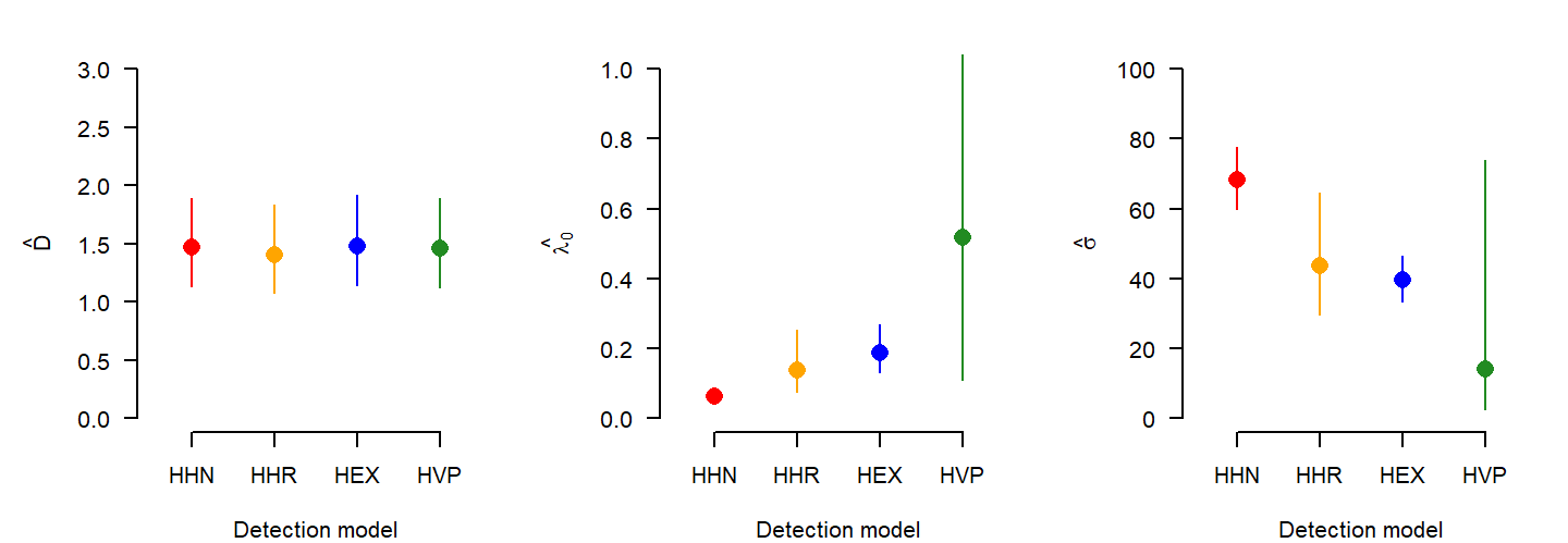
The third parameter z was estimated as 3.08 for HHR, and 0.67 for HVP.

Fitting the HVP function with z fixed to different values is another way to examine the effect of shape (Fig. 10.3). Density estimates ranged only from 1.47 to 1.42.

Figure 10.3: HVP function fitted to snowshoe hare data with z parameter fixed at four different values.

How can different functions produce nearly the same estimates? Remember that \hat D = n/a(\hat \theta), and n is the same for all models. Constant \hat D therefore implies constant effective sampling area a(\hat \theta). In other words, variation in \hat \lambda_0 and \hat \sigma ‘washes out’ when they are combined in a(\hat \theta). Under the four models a(\hat \theta) is estimated as 46.4, 48.4, 45.9 and 46.7 ha.

10.1.2 Detection parameters are mostly nuisance parameters

The detection model and its parameters (g_0, \lambda_0, \sigma etc.) provide the link between our observations and the state of the animal population represented by the parameter D (density, distribution in space, trend etc.). Sub-models for D are considered in Chapter 11. But what interpretation should we attach to the detection parameters themselves?

The intercept g_0 is in a sense the probability that an animal will be detected at the centre of its home range. The spatial scale of detection \sigma relates to the size of the home range. These attributed meanings can aid intuitive understanding. However, we advise against a literal reading. The estimates have meaning only for a specified detection function and cannot meaningfully be compared across functions. Observe the different intercepts of the functions in Fig. 10.2.

The halfnormal function is closest to a standard reference, but estimates of halfnormal \sigma are sensitive to infrequent large movements. Care is also needed because some early writers omitted the factor 2 from the denominator, increasing estimates of \sigma by \sqrt 2⁴.

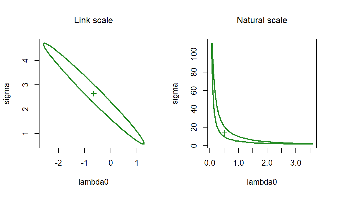
Continuing the snowshoe hare example: the estimates of \lambda_0 and \sigma from HVP are surprisingly uncertain when considered on their own, yet the HVP estimate of density has about the same precision as other detection functions (Fig. 10.2). How can this be? There is strong covariation in the sampling distributions of the two parameters that we plot using ellipse.secr in Fig. 10.4.

Figure 10.4: Confidence ellipse for HVP detection parameters plotted on the link scale and back-transformed to natural scale. ‘+’ indicates MLE.

10.1.3 SECR is not distance sampling

The idea of a distance-detection function originated in distance sampling (Buckland et al., 2001) and Borchers et al. (2015) provided a unified framework for spatially explicit capture–recapture and distance sampling. Nevertheless, the role of the detection function differs substantially.

In distance sampling, shape matters a lot. In particular, the estimate of density depends on the slope of the detection function near the origin, given the assumption that all animals at the origin are detected (e.g., Buckland et al., 2015).

In SECR, no special significance is attached to the intercept or the shape of the function. The detection function serves as a spatial filter for a modelled 2-dimensional point pattern of activity centres; the filter must ‘explain’ the frequency of recaptures and their spatial spread. These are the components of the effective sampling area.

The hazard-rate function HR is recommended for distance sampling because it has a distinct ‘shoulder’ near zero distance, and distance sampling is not concerned with the tail (distant observations are often censored). SECR relies on the tail flattening to zero within the region of integration defined by the habitat mask. Otherwise, the population at risk of detection is determined by the choice of mask, which is usually arbitrary and ad hoc. The hazard-rate function has an extremely long tail (it is not convergent), so there is always a risk of mask-dependence. As an aside - in the snowshoe hare example with detection function HHR we suppressed the warning “predicted relative bias exceeds 0.01 with buffer = 250” that is due to truncation of the long tail.

10.1.4 Why bother?

Given the preceding comments you may wonder why we bother with different detection functions at all. In part this is historical: it was not obvious in the beginning that density estimates were so robust. Sometimes it’s just nice to have the flexibility to match the model to animal behaviour. Functions with longer tails (e.g., HEX) accommodate occasional extreme movements that can prevent a short-tailed function (HHN) from fitting at all.

Also, it is desirable to account for any significant lack of fit due to the detection function before modelling effects that may have a more critical effect on density estimates, such as individual heterogeneity and learned responses.

10.2 Detection submodels

Until now we have assumed that there is a single beta parameter for each real parameter. A much richer set of models is obtained by treating each real parameter as a function of covariates. For convenience, the function is linear on the appropriate link scale. The single ‘beta’ coefficient is then replaced by two or more coefficients (e.g., intercept \beta_0 and slope \beta_1 of the linear relationship y = \beta_0 + \beta_1x_1 where y is a parameter on the link scale and x_1 is a covariate). Suppose, for example, that y depends on sampling occasion s then y(s) = \beta_0 + \beta_1x_1(s) and the corresponding real parameter is y(s) back transformed from the link scale.

This may be generalised using the notation of linear models, \mathbf y = \mathbf X \pmb {\beta}, \tag{10.1}

where \mathbf X is the design matrix, \pmb{\beta} is a vector of coefficients, and \mathbf y is the resulting vector of values on the link scale, one for each row of \mathbf X. The first column of the design matrix is a column of 1’s for the intercept \beta_0. Factor (categorical) predictors will usually be represented by several columns of indicator values (0’s and 1’s coding factor levels). See Cooch & White (2023) Chapter 6 for an accessible introduction to linear models and design matrices.

In secr each detection parameter (g_0, \lambda_0, \sigma, z) is controlled by a linear sub-model on its link scale, i.e. each has its own design matrix. Rows of the design matrix correspond to combinations of session, individual, occasion, and detector, omitting any of these four that is constant (perhaps because there is only one level). Finite-mixture models add further rows to the design matrix that we leave aside for now. Columns after the first are either (i) indicators to represent effects that can be constructed automatically (Table 10.3), or (ii) user-supplied covariates associated with sessions, individuals, occasions or detectors.

Table 10.3: Automatically generated predictor variables for detection models

Variable	Description	Notes
g	group	groups are defined by the individual covariate(s) named in the ‘groups’ argument
t	time factor	one level for each occasion
T	time trend	linear trend over occasions on link scale
b	learned response	step change after first detection
B	transient response	depends on detection at preceding occasion (Markovian response)
bk	animal x site response	site-specific step change
Bk	animal x site response	site-specific transient response
k	site learned response	site effectiveness changes once any animal caught
K	site transient response	site effectiveness depends on preceding occasion
session	session factor	one level for each session
Session	session trend	linear trend on link scale
h2	2-class mixture	finite mixture model with 2 latent classes
ts	marking vs sighting	two levels (marking and sighting occasions)

Each design matrix is constructed automatically when secr.fit is called, using the data and a model formula. Computation of the linear predictor (Eq. 10.1) and back-transformation to the real scale are also automatic: the user need never see the design matrix.

Spatially varying detection

The hard-wired structure of the design matrices precludes some possible sub-models: there is no direct way to model spatial variation in a detection parameter. This was a choice made in the design of the software. It aimed to tame the complexity and resource demands that would result if lambda0, g0 and sigma were allowed to vary continuously in space. However, spatial effects may be modelled efficiently using detector-level covariates, i.e. as a function of detector location rather than AC location, and a further workaround for parameter \sigma is shown in Appendix F.

The formula may be constant (\sim 1, the default) or some combination of terms in standard R formula notation (see ?formula). For example, g0 \sim b + T specifies a model with a learned response and a linear time trend in g0; the effects are additive on the link scale. Table 10.4 has some examples.

Table 10.4: Some examples of the ‘model’ argument in secr.fit

Formula	Effect
g0 \sim 1	g0 constant across animals, occasions and detectors
g0 \sim b	learned response affects g0
list(g0 \sim b, sigma \sim b)	learned response affects both g0 and sigma
g0 \sim h2	2-class finite mixture for heterogeneity in g0
g0 \sim b + T	learned response in g0 combined with trend over occasions
sigma \sim g	detection scale sigma differs between groups
sigma \sim g*T	group-specific trend in sigma

The common question of how to model sex differences can be answered in several ways. we devote Chapter 16 to the possibilities (groups, individual covariate, hybrid mixtures etc.).

Note

Linear sub-models for parameters are considered by Cooch & White (2023) as a constraint on a more general model. Their default is for each parameter to be fully-time-specific e.g., a Cormack-Jolly-Seber open population survival model would fit a unique detection probability p and survival rate \phi at each time. Our default is for each parameter to be constant (i.e. maximally constrained), and for linear sub-models to introduce variation.

10.2.1 Covariates

Any name in a formula that is not listed as a variable in Table 10.3 is assumed to refer to a user-supplied covariate. secr.fit looks for user-supplied covariates in data frames embedded in the ‘capthist’ argument, or supplied in the ‘timecov’ and ‘sessioncov’ arguments, or named with the ‘timevaryingcov’ attribute of a traps object, using the first match (Table 10.5).

Table 10.5: Types of user-provided covariate for parameters of detection models. The names of columns in the respective dataframes may be used in model formulae. Time-varying detector covariates are a special case considered below.

Covariate type	Data source
Individual	covariates(capthist)
Time	timecov argument
Detector	covariates(traps(capthist))
Detector x Time	covariates(traps(capthist))
Session	sessioncov argument

A continuous covariate that takes many unique values poses problems for the implementation in secr. A multiplicity of values inflates the size of internal lookup tables, both slowing down each likelihood evaluation and potentially exceeding the available memory⁵. A binned covariate should do the job equally well, while saving time and space (see function binCovariate).

10.2.2 Time-varying trap covariates

A special mechanism is provided for detector-level covariates that take different values on each occasion. Then we expect the dataframe of detector covariates to include a column for each occasion.

A ‘traps’ object may have an attribute ‘timevaryingcov’ that is a list in which each named component is a vector of indices identifying which covariate column to use on each occasion. The name may be used in model formulae. Use timevaryingcov() to extract or replace the attribute.

10.2.3 Regression splines

Modelling a link-linear⁶ relationship between a covariate and a parameter may be too restrictive.
Regression splines are a very flexible way to represent non-linear responses in generalized additive models, implemented in the R package mgcv (Wood, 2006). Borchers & Kidney (2014) showed how they may be used to model 2-dimensional trend in density. They used mgcv to construct regression spline basis functions from mask x- and y-coordinates, and possibly additional mask covariates, and then passed these as covariates to secr.fit. Smooth, semi-parametric responses are also useful for modelling variation in detection parameters such as g_0 and \sigma over time, or in response to numeric individual- or detector-level covariates, when (1) a linear or other parametric response is arbitrary or implausible, and (2) sampling spans a range of times or levels of the covariate(s).

Smooth terms may be used in secr model formulae for both density and detection parameters. The covariate is merely wrapped in a call to the smoother function s(). Smoothness is controlled by the argument ‘k’.

For a concrete example, consider a population sampled monthly for a year (i.e. 12 ‘sessions’). If home range size varies seasonally then the parameter sigma may vary in a more-or-less sinusoidal fashion. A linear trend is obviously inadequate, and a quadratic is not much better. However, a sine curve is hard to fit (we would need to estimate its phase, amplitude, mean and spatial scale) and assumes the increase and decrease phases are equally steep. An extreme solution is to treat month as a factor and estimate a separate parameter for each level (month). A smooth (semi-parametric) curve may capture the main features of seasonal variation with fewer parameters.

There are some drawbacks to using smooth terms. The resulting fitted objects are large, on account of the need to store setup information from mgcv. The implementation may change in later versions of mgcv and secr, and smooth models fitted now will not necessarily be compatible with later versions. Setting the intercept of a smooth to zero is not a canned option in mgcv, and is not offered in secr. It may be achieved by placing a knot at zero and hacking the matrix of basis functions to drop the corresponding column, plus some more jiggling.

10.2.4 Why bother?

Detailed modelling of detection parameters may be a waste of energy for the same reasons that the choice of detection function itself has limited interest. See, for example, the simulation results of Sollmann (2024) on occasion-specific models (\sim t). However, behavioural responses and individual heterogeneity can have a major effect on density estimates, and these deserve attention.

10.2.4.1 Behavioural responses

An individual behavioral response is a change in the probability or hazard of detection on the occasions that follow a detection. Trapping of small mammals provides evidence of species that routinely become trap happy (presumably because they enjoy the bait) or trap shy (presumably because the experience of capture and handling is unpleasant). Positive or negative responses are modelled as a step change in a detection parameter, usually the intercept of the detection function (g_0, \lambda_0).

The response may be permanent (b) or transient (B) (i.e. applying only on the next occasion). In spatial models we also distinguish between a global response, across all detectors, and a local response, specific to the initial detector (suffix ‘k’). This leads to four response models: b, bk, B, and Bk.

We explore these options with Reid’s Wet Swizer Gulch deer mouse (Peromyscus maniculatus) dataset from Otis et al. (1978). Mice were trapped on a grid of 99 traps over 6 days. The Sherman traps were treated as multi-catch traps for this analysis. We fit the four behavioural response models and the null model to the morning data.

cmod <- paste0('g0~', c('1','b','B','bk','Bk'))
# convert each character string to a formula and fit the models
fits <- list.secr.fit(model = sapply(cmod, formula), constant = 
    list(capthist = 'deermouse.WSG', trace = FALSE, buffer = 80), 
    names = cmod)
AIC(fits, sort = FALSE)[c(3:5,7,8)]

      npar  logLik    AIC    dAIC AICwt
g0~1     3 -663.54 1333.1 129.938     0
g0~b     4 -643.72 1295.4  92.298     0
g0~B     4 -651.62 1311.2 108.099     0
g0~bk    4 -597.57 1203.1   0.000     1
g0~Bk    4 -621.02 1250.0  46.910     0

All response models are preferred to the null model, but the differences among them are marked: the evidence supports a persistent local response (bk). The density estimates for bk and Bk are close to the null model, whereas the b and B estimates are greater. In our experience this is a common result: a local response is preferred by AIC and has less impact on density estimates than a global response, and there is little penalty for omitting the response from the model.

collate(fits, realnames = 'D')[1,,,]

      estimate SE.estimate    lcl    ucl
g0~1    14.089      2.0364 10.629 18.676
g0~b    18.531      3.3459 13.044 26.324
g0~B    15.726      2.3351 11.774 21.005
g0~bk   13.884      2.1108 10.324 18.672
g0~Bk   13.883      2.0472 10.414 18.506

The estimated magnitude of the responses may be examined with predict(fits[2:5], all.levels = TRUE) but the output is long and we show only the global (b) and local (bk) enduring responses:

$`g0~b`
                     estimate   lcl   ucl
session = WSG, b = 0    0.055 0.031 0.096
session = WSG, b = 1    0.210 0.163 0.267

$`g0~bk`
                      estimate   lcl   ucl
session = WSG, bk = 0    0.061 0.044 0.085
session = WSG, bk = 1    0.596 0.454 0.723

Here ‘b = 0’ and ‘bk = 0’ refer to g_0 for a naive animal and ‘b = 1’ and ‘bk = 1’ refer to the post-detection values (estimates are shown with 95% limits). It appears that deermice are highly likely to return to traps where they have been caught.

Detector-level ‘behavioural’ response is also possible (predictors k, K in secr.fit). Detection of any individuals at a detector may in principle be facilitated or inhibited by a previous detection there of any other individual. We are not aware of published examples.

The trap-facilitation model fitted to the deer mouse data results in a larger and less precise estimate of density (16.78/ha, SE 2.59/ha), with AIC intermediate between the null model and bk (facilitation model \DeltaAIC = 73.7 relative to bk). There is a risk of confusing such an effect with simple heterogeneity in the performance of detectors or clumping of activity centres or an individual local response (bk). More investigation is needed.

10.3 Varying effort

Researchers are often painfully aware of glitches in their data gathering - traps that were not set, sampling occasions missed or delayed due to weather etc. Even when the actual estimates are robust, as in an example below, it is desirable (therapeutic and scientific) to allow for known irregularities in the data. This is the role of the ‘usage’ matrix as described in Chapter 3.

The ‘usage’ attribute of a ‘traps’ object in secr is a K x S matrix recording the effort (T_{sk}) at each detector k = 1...K and occasion s = 1...S. Effort may be binary (0/1) or continuous. If the attribute is missing (NULL) it will be treated as all ones. Extraction and replacement functions are provided (usage and usage<-, as demonstrated below). All detector types accept usage data in the same format. The usage matrix for polygon and transect detectors has one row for each polygon or transect, rather than one row per vertex.

Binomial count detectors are a special case. When the secr.fit argument binomN = 1, or equivalently binomN = ‘usage’, usage is interpreted as the size of the binomial distribution (the maximum possible number of detections of an animal at a detector on one occasion).

10.3.1 Input of usage data

Usage data may be input as extra columns in a file of detector coordinates (see ?read.traps and secr-datainput.pdf).

Usage data also may be added to an existing traps object, even after it has been included in a capthist object. For example, the traps object in the demonstration dataset ‘captdata’ starts with no usage attribute, but we can add one. Suppose that traps 14 and 15 were not set on occasions 1–3. We construct a binary usage matrix and assign it to the traps object like this:

K <- nrow(traps(captdata))
S <- ncol(captdata)
mat <- matrix(1, nrow = K, ncol = S)
mat[14:15,1:3] <- 0   # traps 14:15 not set on occasions 1:3
usage(traps(captdata)) <- mat

10.3.2 Models

The usage attribute of a traps object is applied automatically by secr.fit. Following on from the preceding example, we can confirm our assignment and fit a new model.

summary(traps(captdata))    # confirm usage attribute

Object class       traps 
Detector type      single 
Detector number    100 
Average spacing    30 m 
x-range            365 635 m 
y-range            365 635 m 

Usage range by occasion
    1 2 3 4 5
min 0 0 0 1 1
max 1 1 1 1 1

fit <- secr.fit(captdata, buffer = 100, trace = FALSE, biasLimit = NA)
predict(fit)

       link estimate SE.estimate      lcl      ucl
D       log  5.47346    0.645991  4.34659  6.89249
g0    logit  0.27473    0.027164  0.22479  0.33102
sigma   log 29.39668    1.308422 26.94206 32.07494

The result in this case is only subtly different from the model with uniform usage (compare predict(secrdemo.0)). Setting biasLimit = NA avoids a warning message from secr.fit regarding bias.D: this function is usually run by secr.fit after any model fit using the ‘buffer’ argument, but it does not handle varying effort.

Usage is hardwired and will be applied whenever a model is fitted. There are two ways to suppress this. The first is to remove the usage attribute (usage(traps(captdata)) <- NULL). The second is to bypass the attribute for a single fit by calling secr.fit with ‘details = list(ignoreusage = TRUE)’.

For a more informative example, we simulate data from an array of binary proximity detectors (such as automatic cameras) operated over 5 occasions, using the default density (5/ha) and detection parameters (g0 = 0.1, sigma = 25 m) in sim.capthist. We choose to expose all detectors twice as long on occasions 2 and 3 as on occasion 1, and three times as long on occasions 4 and 5:

simgrid <- make.grid(nx = 10, ny = 10, detector = 'proximity')
usage(simgrid) <- matrix(c(1,2,2,3,3), byrow = TRUE, nrow = 100, 
    ncol = 5)
simCH <- sim.capthist(simgrid, popn = list(D = 5, buffer = 100), 
    detectpar = list(g0 = 0.1, sigma = 25), noccasions = 5, 
    seed = 123)
summary(simCH)

Object class       capthist 
Detector type      proximity (5) 
Detector number    100 
Average spacing    20 m 
x-range            0 180 m 
y-range            0 180 m 

Usage range by occasion
    1 2 3 4 5
min 1 2 2 3 3
max 1 2 2 3 3

Counts by occasion 
                    1   2   3   4   5 Total
n                  15  18  23  29  23   108
u                  15   7   6   7   1    36
f                   8   6   9   4   9    36
M(t+1)             15  22  28  35  36    36
losses              0   0   0   0   0     0
detections         26  32  39  54  55   206
detectors visited  24  28  33  41  44   170
detectors used    100 100 100 100 100   500

Now we fit four models with a half-normal detection function. The firest model (fit.null) has no adjustment because we ignore the usage information. The second (fit.usage) automatically adjusts for effort. The third (fit.tcov1) again ignores effort, but fits a distinct g0 for each level of effort. The fourth (fit.tcov2) uses a numerical covariate equal to the known effort. The setting fastproximity = FALSE allows all models can be compared by AIC.

# shared arguments for model fits 1-4
timedf <- data.frame(tfactor = factor(c(1,2,2,3,3)), tnumeric = 
    c(1,2,2,3,3))
args <- list(capthist = simCH, buffer = 100, biasLimit = NA, 
    timecov = timedf, trace = FALSE)
models <- c(g0 ~ 1, g0 ~ 1, g0 ~ tfactor, g0 ~ tnumeric)
details <- rep(list(list(ignoreusage = TRUE, fastproximity = 
    FALSE)), 4)
details[[2]]$ignoreusage <- FALSE

# review arguments
data.frame(model = format(models), ignoreusage = sapply(details,
    '[[', 'ignoreusage'))

          model ignoreusage
1        g0 ~ 1        TRUE
2        g0 ~ 1       FALSE
3  g0 ~ tfactor        TRUE
4 g0 ~ tnumeric        TRUE

# fit
fits <- list.secr.fit(model = models, details = details, constant = 
    args, names = c('null','usage','tfactor','tnumeric'))
AIC(fits)[,-c(2,5,6)]

                           model npar  logLik   dAIC  AICwt
usage           D~1 g0~1 sigma~1    3 -737.20  0.000 0.4212
tnumeric D~1 g0~tnumeric sigma~1    4 -736.24  0.072 0.4063
tfactor   D~1 g0~tfactor sigma~1    5 -736.09  1.785 0.1725
null            D~1 g0~1 sigma~1    3 -744.90 15.390 0.0000

From the likelihoods we can see that failure to allow for effort (model ‘null’) dramatically reduces model fit. The model with a factor covariate (‘tfactor’) captures the variation in detection probability, but at the cost of fitting two additional parameters. The model with built-in adjustment for effort (‘usage’) has AIC similar to one with effort as a numeric covariate (‘tnumeric’). How do the estimates compare? This is a task for the collate function.

collate(fits, newdata = timedf)[,,'estimate','g0']

                        null   usage tfactor tnumeric
tfactor=1,tnumeric=1 0.21001 0.10112 0.13349  0.12551
tfactor=2,tnumeric=2 0.21001 0.10112 0.18047  0.18851
tfactor=2,tnumeric=2 0.21001 0.10112 0.18047  0.18851
tfactor=3,tnumeric=3 0.21001 0.10112 0.27772  0.27324
tfactor=3,tnumeric=3 0.21001 0.10112 0.27772  0.27324

The ‘null’ model fits a single g0 across all occasions that is approximately twice the true rate on occasion 1 (0.1). The estimates of g0 from ‘tfactor’ and ‘tnumeric’ mirror the variation in effort. The effort-adjusted ‘usage’ model estimates the fundamental rate for one unit of effort (0.1).

collate(fits)[,,,'D']

         estimate SE.estimate    lcl    ucl
null       4.9709     0.84830 3.5663 6.9287
usage      4.9755     0.84881 3.5700 6.9344
tfactor    4.9703     0.84811 3.5660 6.9277
tnumeric   4.9698     0.84805 3.5656 6.9271

The density estimates themselves are almost entirely unaffected by the choice of model for g0. This is not unusual (Sollmann, 2024). Nevertheless, the example shows how ‘usage’ allows unbalanced data to be analysed with a minimum of fuss.

10.3.3 Further notes on varying effort

1. Adjustment for varying effort will be more critical in analyses where (i) the variation is confounded with temporal (between-session) or spatial variation in density, and (ii) it is important to estimate the temporal or spatial pattern. For example, if detector usage was consistently high in one part of a landscape, while true density was constant, failure to allow for varying usage might produce a spurious density pattern.
2. The units of usage determine the units of g_0 or \lambda_0 in the fitted model. This must be considered when choosing starting values for likelihood maximization. Ordinarily one relies on secr.fit to determine starting values automatically (via autoini), and a simple linear adjustment for usage, averaged across non-zero detectors and occasions, is applied to the value of g0 from autoini.
3. When occasions are collapsed or detectors are lumped with the reduce method for capthist objects, usage is summed for each aggregated unit.
4. The function usagePlot displays a bubble plot of spatially varying detector usage on one occasion. The arguments ‘markused’ and ‘markvarying’ of plot.traps may also be useful.
5. Absolute duration does not always equate with effort. Animal activity may be concentrated in part of the day, or older DNA samples from hair snares may fail to amplify (Efford et al., 2013).
6. Binary or count data from searches of polygons or transects (Efford, 2011) do not raise any new issues for including effort, at least when effort is homogeneous across each polygon or transect. Effects of varying polygon or transect size are automatically accommodated in the models of Chapter 4. Models for varying effort within polygons or transects have not been needed for problems encountered to date. Such variation might in any case be accommodated by splitting the searched areas or transects into smaller units that were more nearly homogeneous (see the snip function for splitting transects).

Borchers, D. L., & Kidney, D. (2014). Flexible density surface estimation for spatially explicit capture–recapture surveys. University of St Andrews. https://research-repository.st-andrews.ac.uk/bitstream/handle/10023/9147/secrgam_techrep.pdf?sequence=1

Borchers, D. L., Stevenson, B. C., Kidney, D., Thomas, L., & Marques, T. A. (2015). A unifying model for capture–recapture and distance sampling surveys of wildlife populations. Journal of the American Statistical Association, 110(509), 195–204. https://doi.org/10.1080/01621459.2014.893884

Buckland, S. T., Anderson, D. R., Burnham, K. P., Laake, J. L., Borchers, D. L., & Thomas, L. (2001). Introduction to distance sampling. Oxford University Press.

Buckland, S. T., Rexstad, E. A., Marques, T. A., & Oedekoven, C. S. (2015). Distance sampling: Methods and applications. Springer.

Cooch, E., & White, G. (Eds.). (2023). Program MARK: A gentle introduction. (23rd ed.). http://www.phidot.org/software/mark/docs/book/

Efford, M. G. (2011). Estimation of population density by spatially explicit capture-recapture analysis of data from area searches. Ecology, 92, 2202–2207.

Efford, M. G., Borchers, D. L., & Mowat, G. (2013). Varying effort in capture-recapture studies. Methods in Ecology and Evolution, 4, 629–636.

Ergon, T., & Gardner, B. (2013). Separating mortality and emigration: Modelling space use, dispersal and survival with robust‐design spatial capture–recapture data. Methods in Ecology and Evolution, 5(12), 1327–1336. https://doi.org/10.1111/2041-210x.12133

Gardner, B., Royle, J. A., & Wegan, M. T. (2009). Hierarchical models for estimating density from DNA mark-recapture studies. Ecology, 90, 1106–1115.

Hayes, R. J., & Buckland, S. T. (1983). Radial-distance models for the line-transect method. Biometrics, 39, 29–42.

Kendeigh, S. C. (1944). Measurement of bird populations. Ecological Monographs, 14, 67–106. https://doi.org/10.2307/1961632

Otis, D. L., Burnham, K. P., White, G. C., & Anderson, D. R. (1978). Statistical inference from capture data on closed animal populations. Wildlife Monographs, 62.

Royle, J. A., Chandler, R. B., Sollmann, R., & Gardner, B. (2014). Spatial capture-recapture. Academic Press.

Royle, J. A., Chandler, R. B., Sun, C. C., & Fuller, A. K. (2013). Integrating resource selection information with spatial capture–recapture. Methods in Ecology and Evolution, 4(6), 520–530. https://doi.org/10.1111/2041-210x.12039

Royle, J. A., Fuller, A. K., & Sutherland, C. (2015). Spatial capture–recapture models allowing markovian transience or dispersal. Population Ecology, 58(1), 53–62. https://doi.org/10.1007/s10144-015-0524-z

Royle, J. A., & Gardner, B. (2011). Hierarchical spatial capture-recapture models for estimating density from trapping arrays. In A. F. O’Connell, J. D. Nichols, & K. U. Karanth (Eds.), Camera traps in animal ecology: Methods and analyses (pp. 163–190). Springer.

Royle, J. A., Magoun, A. J., Gardner, B., Valkenburg, P., & Lowell, R. E. (2011). Density estimation in a wolverine population using spatial capture-recapture models. Journal of Wildlife Management, 75, 604–611.

Sollmann, R. (2024). Mt or not mt: Temporal variation in detection probability in spatial capture-recapture and occupancy models. Peer Community Journal, 4. https://doi.org/10.24072/pcjournal.357

Wood, S. N. (2006). Generalized additive models: An introduction with R. Chapman; Hall/CRC.

---

1. The transformation is non-linear so, for example, a half-normal form for g(.) does not correspond to half-normal form for \lambda(.).

2. This use of ‘hazard’ has historical roots in distance sampling (Hayes & Buckland, 1983) and has no real connection to models for hazard as a function of distance.

3. Technically this is the cumulative hazard rather than the instantaneous hazard, but we get tired of using the full term.

4. Examples are Gardner et al. (2009), Royle & Gardner (2011) and Royle et al. (2011), but not Royle et al. (2014) and Royle et al. (2015)).

5. In the C++ code, two real-valued 3-dimensional arrays are populated with pre-computed values of p_{sk}(\mathbf x) (gk) and h_{sk}(\mathbf x) (hk). The dimensions are the number of unique parameter combinations C, the number of detectors K and the number of mask points M. The memory requirement for these arrays alone is 2.8.C.K.M bytes, which for 200 detectors, 10000 mask points, and 100 parameter levels is 3.2 Gb. This is on top of the two parameter index arrays requiring 2 . 4 . R. n. S. K. U bytes for R sessions and U mixture classes (e.g. 10 sessions, 200 animals, 6 occasions, 200 detectors and 2 mixture classes, 0.0384 Gb), and a number of smaller objects.

6. We use ‘link-linear’ to describe a linear model on the link scale, where this may be log-linear, logit-linear etc.