Appendix E — Mark-resight models

E.1 How is mark-resight different?

In capture–recapture, all newly detected unmarked animals become marked and are distinguishable in future. Some field protocols also involve ‘resighting’ occasions on which previously marked animals are identified but newly detected animals are not marked. We call these ‘mark–resight’ data. McClintock & White (2012) provide an excellent summary of non-spatial mark–resight methods. The extension of spatially explicit capture–recapture models for mark–resight data was begun by Sollmann et al. (2013), and spatial mark–resight models were applied by Rich et al. (2014) and Rutledge et al. (2015). Whittington et al. (2018) describe a major Bayesian application.

E.2 Distribution of marked animals

The historical development of mark–resight models has stressed the resighting component of mark–resight data; the sampling process leading to marking is not modelled. Modelling of the sighting data then requires some assumption about the distribution of the marked animals. Most commonly, marked animals are assumed to be a random sample from a defined population, and that may be achievable in some situations. An important case is when some animals carry natural marks and others don’t, as in the puma study of Rich et al. (2014).

However, when a spatially distributed population is sampled with localized detectors such as traps, animals living near the traps have a higher chance of becoming marked, and the marked animals are not representative of a well-defined population. The difficulty may be overcome by spatially modelling both the marking and resighting processes. This requires that data on detection locations were collected during the marking phase, and that the spatial distribution of marking effort was recorded. Matechou et al. (2013) analysed non-spatial capture–recapture–resighting data jointly with counts of unmarked individuals, and the core capture–mark–resight models in secr are their spatial equivalent (see also Whittington et al. (2018)).

Rather than modelling the marking process we may take the traditional path, i.e. assume a certain spatial distribution for the marked individuals. Typically, the distribution is assumed to be uniform over a known area (e.g., Sollmann et al. (2013), Rich et al. (2014)). The number of marked individuals remaining at the time of resighting may be known or unknown. We use ‘capture–mark–resight’ for models that include the marking process and ‘sighting-only’ for models in which the spatial distribution of marks is assumed.

E.3 Overview of implementation in secr

The implementation in secr follows Efford & Hunter (2018). The models discard some spatial information in the unmarked sightings – information that is used in the models of Chandler & Royle (2013) and Sollmann et al. (2013). This results in some (probably small) loss of precision, and requires an adjustment for overdispersion to ensure confidence intervals have good coverage properties.

Following Efford & Hunter (2018),

• the population is assumed to follow a (possibly inhomogeneous) Poisson distribution in space
• detection histories of marked animals are modelled as usual in SECR
• counts of unmarked sightings are modelled with a Poisson distribution
• overdispersion in the counts (relative to a Poisson distribution) is estimated by simulation and used in a pseudo-likelihood estimate. The adjustment has minimal effect on the estimates themselves, but improves coverage of confidence intervals

Unidentified sightings of marked animals are treated as independent of identified sightings. This is an approximation, but its effect on estimates is believed to be negligible.

The core models are listed in Table E.1. These may be customized in various ways, particularly by specifying the assumed distribution of marked animals for sighting-only models. Each model may be fitted with or without a parameter for incomplete identification of marked animals when they are resighted (pID).

Table E.1: Classification of mark–resight models available in secr. ‘Capture–mark–resight’ models include the marking process; ‘sighting-only’ models rest on prior knowledge or assumptions regarding where animals have been marked. For sighting-only data some detection histories may be all-zero.

Data	Pre-marking1	Code
Capture–mark–resight	none	NA
Sighting-only	Known n_0	details = list(knownmarks = TRUE)
	Unknown n_0	details = list(knownmarks = FALSE)

1. n_0 is the number of marked individuals in the study area at the time of the sighting surveys.

Mark–resight data are represented in secr by a capthist data object, with minor extensions (Table E.2). We describe the structure for a single-session capthist object, which records detections of each marked animal over S occasions at any of K detectors. Detectors on sighting occasions may be of the usual binary proximity (‘proximity’) or count proximity (‘count’) types¹. Detectors on marking occasions may be any combination of these types and multi-catch traps. Area search (‘polygon’) and transect search (‘transect’) types are not yet supported for either phase when there are sighting occasions: discretization is recommended.

Warning

Not all detector types and options in secr will work with mark–resight data. See Limitations for a list of known constraints (some will be mentioned along the way). See the step-by-step guide for a quick introduction.

Table E.2: Special attributes of data objects for mark–resight analysis in secr.

Object	Attribute	Description
traps	markocc	Occasions may be marking (1), sighting (0) or unresolved (-1)
capthist	Tu	Counts of unmarked animals
capthist	Tm	Counts of marked animals not identified
capthist	Tn	Counts of sightings with unknown mark status (not modelled)
mask	marking1	Distribution of pre-marked animals (sighting-only data; optional)

1. marking is the name of a special mask covariate, accessed like other covariates.

E.3.1 Marking and sighting occasions

Sampling occasions (intervals) are either marking occasions or sighting occasions. On marking occasions any recaptured animals are also recorded². On sighting occasions newly caught animals are released unmarked. The body of the capthist object has one row for each individual detected on at least one marking occasion, and one column for each occasion, whether marking or sighting.

The ‘traps’ object, a required attribute of any capthist object, has its own optional attribute markocc to distinguish marking occasions (1) from sighting occasions (0) (e.g., c(1,0,0,0,0) for marking on one occasion followed by four resighting occasions). A capthist object is recognised as a mark–resight dataset if its traps has a markocc attribute with at least one sighting occasion (i.e. !all(markocc)). Marking occasions and sighting occasions may be interspersed.

E.3.2 Sighting-only data

A sighting-only dataset has a markocc attribute with no marking occasions. Two scenarios are possible: either the capthist object includes a sighting history for each marked animal (including all-zero histories for any not re-sighted), or it includes sighting histories only for the re-sighted animals. In the latter case the number of marked animals at the time of sampling is unknown, and the fitted model must take account of this (see Number of marks unknown).

E.3.3 Sightings of unmarked animals

In addition to the marking and sighting events of known individuals recorded in the body of the capthist object, there will usually be sightings of unmarked animals. These data take the form of a matrix with the number of detections of unmarked animals at each detector (row) on each sampling occasion (column). A single searched polygon or transect is one detector and hence contributes a single row. Columns corresponding to marking occasions are all-zero. This matrix is stored as attribute Tu of the capthist object.

Instead of providing Tu as a matrix, the counts may be summed over occasions (Tu is a vector of detector-specific counts), or provided as the grand total (Tu is a single integer). These alternatives have definite limitations:

• occasion-specific or detector-specific models cannot be fitted
• plot, summary and verify are less informative
• cannot subset by occasion or detector
• AIC should not be used compare models differing in summarisation
• cannot mix markocc -1 and 0

E.3.4 Unidentified sightings of marked animals

An observer may be able to to determine that an animal is marked, but be unable to positively identify it as a particular individual. The number of sightings of marked but unidentified individuals is stored as capthist attribute Tm, which uses the same formats as Tu.

E.3.5 Sightings of unknown status

Sightings for which the mark status could not be determined are a further category of sighting on sighting occasions. For example, the identifying mark may not be visible in a photograph because of the orientation the animal. The number of sightings with unknown mark status is generally not used in the models (but see unresolved sightings). However, it is good practice to account for these observations. They may be stored as capthist attribute Tn and will appear in summaries.

E.3.6 Unresolved sightings

Sometimes the sighting method does not allow marked animals to be distinguished from unmarked animals. Sighting occasions of this type are coded with ‘-1’ in the markocc vector. On these occasions the counts of all sightings (‘unresolved sightings’) stored in the appropriate column of Tn, the corresponding columns of Tu and Tm are all-zero, and no sightings of marked animals appear in the capthist object. Models comprising one or more marking occasions and only unresolved sightings (e.g., markocc <- c(1, -1, -1, -1, -1)) may be fitted in secr, but there are constraints (see Sighting without attention to marking).

E.4 Data preparation

Data on marked animals may be formatted and read as usual with read.capthist (secr-datainput.pdf). Each identified sighting of a marked individuals appears as a row in the ‘capture’ file, like any other detection. The markocc attribute may be set as an argument of read.capthist or assigned later.

Sighting data for unmarked animals (Tu) are provided separately as a K \times S matrix, where K is the number of detectors and S is the total number of occasions (including marking occasions). Elements in the matrix are either binary (0/1) for proximity detectors, or whole numbers (0, 1, 2,…) for count, polygon and transect detectors. Sightings of marked animals that are not identified to individual (Tm) are optionally provided in a separate K \times S matrix. Usually you will read these data from separate text files or spreadsheets. Sightings with unknown mark status (Tn) may also be provided, but will be ignored in analyses except for occasions with code -1 in markocc.

The function addSightings may be used to merge these matrices of sighting data with an existing mark–resight capthist object, i.e. to set its attributes Tu and Tm. There are also custom extraction and replacement functions for sighting-related attributes (markocc, Tu and Tm). addSightings also allows input from text files in which the first column is a session identifier (see Step-by-step guide for an example).

Let’s assume you have prepared the files MRCHcapt.txt, MRCHcapt.txt, Tu.txt and Tm.txt. Simulated examples can be found in the extdata folder of the secr distribution (version 4.4.3 and above). This code can be used to build a mark–resight capthist object:

library(secr)
olddir <- setwd(system.file("extdata", package = "secr"))
MRCH <- read.capthist("MRCHcapt.txt", "MRCHtrap.txt", detector = 
    c("multi", rep("proximity",4)), markocc = c(1,0,0,0,0))
MRCH <- addSightings(MRCH, "Tu.txt", "Tm.txt")
session(MRCH) <- "Simulated mark-resight data"
setwd(olddir)

E.4.1 Data summary

The summary method for capthist objects recognises mark–resight data and provides a summary of the markocc, Tu, and Tm attributes.

summary(MRCH)

Object class       capthist 
Detector type      multi, proximity (4) 
Detector number    36 
Average spacing    20 m 
x-range            0 100 m 
y-range            0 100 m 

Marking occasions
 1 2 3 4 5
 1 0 0 0 0

Counts by occasion 
                   1  2  3  4  5 Total
n                 70 15 16 19 17   137
u                 70  0  0  0  0    70
f                 28 24 13  3  2    70
M(t+1)            70 70 70 70 70    70
losses             0  0  0  0  0     0
detections        70 17 18 28 23   156
detectors visited 31 14 15 18 13    91
detectors used    36 36 36 36 36   180

Sightings by occasion 
          1  2  3  4  5 Total
ID        0 17 18 28 23    86
Not ID    0  8  5 11  7    31
Unmarked  0  7  9  6  9    31
Uncertain 0  0  0  0  0     0
Total     0 32 32 45 39   148

The main table of counts is calculated differently for sighting-only and capture–mark–resight data. When markocc includes marking occasions the counts refer to marking, recaptures and sightings of marked animals. This means that u (number of new individuals) is always zero on sighting occasions, and M(t+1) increases only on marking occasions. When markocc records that the data are sighting-only, the main table of counts summarises identified sightings of previously marked animals, accumulating u and M(t+1) as if all occasions were marking occasions.

On sighting occasions the row ‘detections’ in Counts by occasion corresponds to the number of sightings of marked and identified individuals (‘ID’) in Sightings by occasion. Other detections in the sightings table are additional to the main table.

The default plot of a mark–resight capthist object shows only marked and identified individuals. To make a separate plot of the sightings of unmarked individuals, either use the same function with type = "sightings" or use sightingPlot:

par(mar = c(1,3,3,3), mfrow = c(1,2), pty = 's')
# petal plot with key
plot(MRCH, type = "sightings", border = 20)
occasionKey(MRCH, cex = 0.7, rad = 5, px = 0.96, py = 0.88, 
            xpd = TRUE)
# bubble plot
sightingPlot(MRCH, "Tu", mean = FALSE, border = 20, fill = TRUE, 
    col = "blue", legend = c(1,2,3), px = 1.0, py = c(0.85,0.72),
    xpd = TRUE)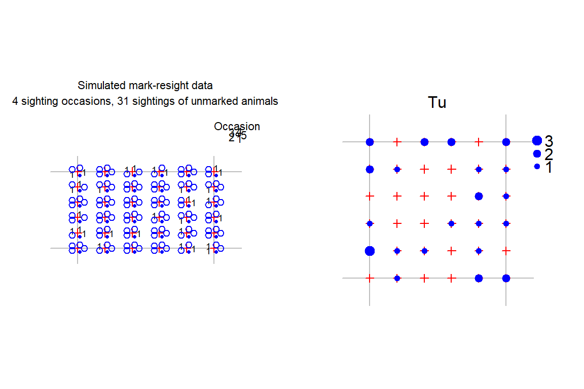

Figure E.1: Two ways to plot sightings of unmarked animals. Petals in the lefthand plot indicate the number of sightings, except that marking occcasions are shown as a solid dot. mean = FALSE causes sightingPlot to use the total over all occasions rather than the mean. Other settings are used here only to customise the layout and colour of the plots.

E.4.2 Data checks

The verify method for capthist objects checks that mark–resight data satisfy

• the length of markocc matches the number of sampling occasions S
• animals are not marked on sighting occasions, or sighted on marking occasions
• the dimensions of matrices with counts of sighted animals (Tu, Tm) match the rest of the capthist object
• sightings are made only when detector usage is > 0
• counts are whole numbers.

Checks are performed by default when a model is fitted with secr.fit, or when verify is called independently.

E.4.3 Different layouts for marking and sighting

Detector layouts are likely to differ between marking and sighting occasions. This can be accommodated within a single, merged detector layout using detector- and occasion-specific usage codes. See here for a function to create a single-session mark–resight traps object from two components.

E.4.4 Simulating mark–resight data

Mark–resight data may be generated with function sim.resight. In this example, one grid of detectors is used for both marking and for resighting, but the detection rate is higher on the initial (marking) occasion.

grid <- make.grid(detector = c("multi", rep("proximity",4)))
markocc(grid) <- c(1, 0, 0, 0, 0)
g0mr <- c(0.3, 0.1, 0.1, 0.1, 0.1)
simMRCH <- sim.resight(grid, detectpar=list(g0 = g0mr, sigma = 25),  
    popn = list(D = 30), pID = 0.7)

If all elements of markocc are zero then a separate mechanism is used to pre-mark a fraction pmark of individuals selected at random from the population. The resulting sighting-only data may include all-zero sighting histories for marked animals. Use the argument markingmask to simulate marking of animals with centres in a certain subregion.

E.4.5 Input of sighting-only data

For sighting-only data we postulate that the marked animals are a random sample of individuals from a known spatial distribution, possibly a specified region. The body of the capthist object then comprises sightings of known individuals, with other sightings in attributes Tu and Tm. Marked animals that were known to be present but not resighted are included as ‘all-zero’ detection histories in the body of the capthist object. These detection histories are input by including a record in the detection file for each marked-but-unsighted individual, distinguished by 0 (zero) in the ‘occasion’ field, and with an arbitrary (but not missing) detector ID or coordinates in the next field(s).

E.5 Model fitting

Properly prepared, a capthist object includes all the data for fitting a mark–resight model³. It is only necessary to call secr.fit. Here is an example in which we use a coarse mask (nx = 32 instead of the default nx = 64) to speed things up. The predictor ‘ts’ and the new ‘real’ parameter pID are explained in following sections.

mask <- make.mask(traps(MRCH), nx = 32, buffer = 100)
fit0 <- secr.fit(MRCH, model = list(g0 ~ ts), mask = mask, 
    trace = FALSE)
predict(fit0, newdata = data.frame(ts = factor(c("M","S"))))

$`ts = M`
       link estimate SE.estimate      lcl      ucl
D       log 25.87863    3.410206 20.01037 33.46783
g0    logit  0.37635    0.053074  0.27923  0.48454
sigma   log 25.30921    1.972903 21.72832 29.48024
pID   logit  0.67424    0.054842  0.55923  0.77150

$`ts = S`
       link  estimate SE.estimate      lcl      ucl
D       log 25.878634    3.410206 20.01037 33.46783
g0    logit  0.093003    0.012526  0.07119  0.12063
sigma   log 25.309209    1.972903 21.72832 29.48024
pID   logit  0.674239    0.054842  0.55923  0.77150

This example relies on the built-in autoini function to provide starting parameter values for the numerical maximization. However, the automatic values may not work with complex mark–resight models. It is not worth continuing if the first likelihood evaluation fails, as indicated by LogLik NaN when trace = TRUE. Then you should experiment with the start argument until you find values that work.

E.5.1 Adjustment for overdispersion

The default confidence intervals have poor coverage when the data include counts in Tu or Tm. This is due to overdispersion of the summed counts, caused by a quirk of the model specification: covariation is ignored in the multivariate Poisson model used to describe the counts. A simple protocol fixes the problem:

1. Fit a model assuming no overdispersion,
2. Estimate the overdispersion by simulating at the initial estimates, and
3. Re-fit the model (or at least re-estimate the variance-covariance matrix) using an overdispersion-adjusted pseudo-likelihood.

Steps (2) and (3) may be performed together in one call to secr.fit. In the example below, the first line repeats the model specification, while the second line provides the previously fitted model as a starting point and calls for nsim simulations to estimate overdispersion (c-hat in MARK parlance).

fit1 <- secr.fit(MRCH, model = list(g0~ts), mask = mask, 
    trace = FALSE, start = fit0, details = list(nsim = 10000))

sims completed

predict(fit1, newdata = data.frame(ts = factor(c("M","S"))))

$`ts = M`
       link estimate SE.estimate      lcl      ucl
D       log 24.13195    3.392929 18.34423 31.74573
g0    logit  0.44590    0.077217  0.30368  0.59755
sigma   log 25.55800    2.037723 21.86596 29.87343
pID   logit  0.66675    0.064273  0.53160  0.77910

$`ts = S`
       link  estimate SE.estimate       lcl      ucl
D       log 24.131951    3.392929 18.344231 31.74573
g0    logit  0.094439    0.013448  0.071174  0.12429
sigma   log 25.557999    2.037723 21.865962 29.87343
pID   logit  0.666747    0.064273  0.531598  0.77910

For this dataset the adjustment had a small effect on the confidence intervals (0% increase in interval length). The estimates of overdispersion are saved in the details$chat component of the fitted model, and we can see that they are close to 1.0. Note that the adjustment is strictly for overdispersion in the unmarked sightings, and the effect of that overdispersion is ‘diluted’ by other components of the likelihood.

fit1$details$chat[1:2]

    Tu     Tm 
1.9651 1.6944 

A shortcut is to specify method = "none" at Step 3 to block re-maximization of the pseudolikelihood: then only the variance-covariance matrix, likelihood and related parameters will be re-computed. Pre-determined values of \hat c may be provided as input in the chat component of details; if nsim = 0 the input chat will be used without further simulation (example in Step-by-step guide Step 8).

Stochasticity in the estimate of overdispersion causes parameter estimates to vary. The problem is minimized by running many simulations (say, nsim = 10000), which has relatively little effect on total execution time.

CAVEAT: the multi-threaded simulation code does not allow for potential non-independence of random number streams across threads. If this is a concern then set ncores = 1 to block multi-threading. See also ?secrRNG.

E.5.2 Different parameter values on marking and sighting occasions

Marking and sighting occasions share parameters by default. This may make sense for the spatial scale parameter (sigma ~ 1), but it is unlikely to hold for the baseline rate (intercept) g0 or lambda0. Density estimates can be very biased if the difference is ignored⁴. A new canned predictor ‘ts’ is introduced to distinguish marking and sighting occasions. For example g0 ~ ts will fit two levels of g0, one for marking occasions and one for sighting occasions. The same can be achieved with g0 ~ tcov, timecov = factor(2-markocc).

To see the values associated with each level of ‘ts’ (i.e., marking and sighting occasions) we specify the newdata argument of predict.secr, as in Adjustment for overdispersion.

E.5.3 Proportion identified

If some sightings are of marked animals that cannot be identified to individual then a further ‘real’ parameter is required for the proportion identified. This is called pID in secr. pID is estimated by default, whether or not the capthist object has attribute Tm, because failure to identify marked animals affects the re-detection probability of marked individuals. For data with a single initial marking occasion, a model estimating pID is exactly equivalent to a learned response model (g0 ~ b) in the absence of Tm (same density estimate, same likelihood).

pID may be fixed at an arbitrary value, just like other real parameters. For example, a call to secr.fit with fixed = list(pID = 1.0) implies that every sighted individual that was already marked could be identified.

Only a subset of the usual predictors is appropriate for pID. Use of predictors other than session, Session, or the names of any session or trap covariate will raise a warning.

E.5.4 Specifying distribution of pre-marked animals (sighting-only models)

By default, animals in a sighting-only dataset are assumed to have been marked throughout the habitat mask. However, uniform marking across a subregion of the habitat mask, or any other known distribution, may be specified by including a mask covariate named ‘marking’. For example,

mask <- make.mask(grid)
d <- distancetotrap(mask, grid)
covariates(mask) <- data.frame(marking = d < 60)

If the mask is used in secr.fit with a sighting-only dataset, the fitted model will ‘understand’ that animals centred within 60 m of the grid had a uniform probability of marking, and no animals from beyond this limit were marked. Note that the area is supposed to contain the centres of all marked animals; this is not the same as a searched polygon. If the covariate is missing then all animals in the mask are assumed to have had an equal chance of becoming marked. The ‘marking’ covariate is actually more general, in that it can represent any known or assumed probability distribution for the locations of marked animals within the mask: values are automatically normalized by dividing by their sum. Be warned that assumptions about the extent of marking directly affect the estimated density.

It is possible in principle that the marked animals are distributed over an area larger than the habitat mask. The software does not directly allow for this. An easy solution is to increase the size of the habitat mask, but take care to control its coarseness (spacing), and be aware of the effect on estimates of N, and on the sampling variance if distribution = "binomial".

E.5.5 Number of marks unknown (sighting-only models)

Sighting-only datasets may entail the further complication that the number of marked animals in the population at the time of resighting is unknown (Model 3). This can happen if enough time has passed for some marked animals to have died or emigrated. It also arises if individuation relies on unique natural marks, but these are missing from some individuals (Rich et al. 2014).

The resighting data do not include any all-zero detection histories, as the only way to know for certain that a marked animal is still present is to sight it at least once. The theory nevertheless allows a spatial model to be fitted⁵.

Data preparation is exactly as for sighting-only models with known number of marks, except that there are no all-zero histories. The unknown-marks model is fitted by setting the secr.fit argument details = list(knownmarks = FALSE), (possibly along with other details components).

E.5.6 Covariates, groups and finite mixtures

Conditional-likelihood models are generally not useful for mark-resight analyses. Individual covariates therefore should not be used in mark-resight models in secr. Other covariates (at the level of session, occasion, or detector) should work in any of the models.

The mark–resight models in secr do not currently allow groups (g). Finite mixtures, including ‘hcov’ models, are only partly implemented.

E.5.7 Discarding unmarked sightings

Sighting data can be highly problematic because of difficulty in reading marks and determining when consecutive sightings are independent. A conservative approach is to discard the counts of unmarked sightings (Tu) and unidentified marked animals (Tm), while retaining sighting data on marked animals. This works for capture–mark–resight data (marking occasions included), but not for all-sighting data (which rely on unmarked sightings to estimate detection parameters). The parameter pID is confounded with the sighting-phase g0 so we fix it at 1.0. The likelihood does not require adjustment for overdispersion of unmarked sightings.

Tu(MRCH) <- NULL
Tm(MRCH) <- NULL
mask <- make.mask(traps(MRCH), nx = 32, buffer = 100)
fit2 <- secr.fit(MRCH, model = list(g0~ts), fixed = list(pID = 1.0), 
    mask = mask, trace = FALSE)
predict(fit2, newdata = data.frame(ts = factor(c("M","S"))))

$`ts = M`
       link estimate SE.estimate       lcl      ucl
D       log  18.1896     2.96621 13.241198 24.98738
g0    logit   0.9446     0.15068  0.056934  0.99979
sigma   log  26.8962     2.32809 22.706517 31.85902

$`ts = S`
       link  estimate SE.estimate       lcl       ucl
D       log 18.189635   2.9662052 13.241198 24.987378
g0    logit  0.063549   0.0088513  0.048255  0.083266
sigma   log 26.896234   2.3280869 22.706517 31.859020

Confidence interval length has increased by -12% over the full estimates (we did throw out a lot of data), but we expect the result to be more robust.

E.5.8 Comparing models

Fitted models may be compared by AIC or AICc. Models can be compared when they describe the same data. In practice this means

1. Do not compare models with and without either sighting attribute (Tu, Tm), and

2. Do not compare sighting-only models with different pre-marking assumptions (the marking covariate of the mask).

E.6 Limitations

These limitations apply when fitting mark–resight models in secr:

• only ‘multi’, ‘proximity’ and ‘count’ detector types are allowed
• groups (g) are not allowed
• hybrid mixtures with known class membership (‘hcov’) have not been implemented for mark-resight data
• some secr functions do not yet handle mark–resight data or models. These are mostly flagged with a Warning on their documentation page.

If the sighting phase is an area or transect search then it may be possible to analyse the data by rasterizing the areas or transects (function discretize).

E.6.1 Warning

The implementation of spatially explicit mark–resight models is still somewhat limited. It is intended that mark–resight models work across other capabilities of secr, particularly

• data may span multiple sessions (multi-session capthist objects can contain mark–resight data)
• mark–resight may be augmented with telemetry data (addTelemetry), but joint telemetry models have not been tested and should be used with care
• fxiContour() and related functions (probability density plots of centres of detected animals)
• finite mixture (h2) models are allowed for detection parameters, including pID
• modelAverage() and collate()
• linear habitat masks are allowed (as in the package secrlinear)

However, these uses have not been tested much, where they have been tested at all..

It is unclear what sample size should be used for sample-size-adjusted AIC (AICc). This is one more reason to use AIC(..., criterion = "AIC"). Currently secr uses the number of detection histories of marked individuals, as for other models.

E.6.2 Pitfalls

The likelihood for the sighting-only model with unknown number of marks (Model 3) has a boundary corresponding to the density of detected marks in the marking mask (true density cannot be less than this). This is ordinarily not a problem (estimated density will usually be larger). However, for multi-session data with a common density parameter it is quite possible for the number of marks in a particular session to exceed the threshold. The log-likelihood function then returns ‘NA’; although maximization may proceed, variance estimation is likely to fail. A possible (but slow) workaround is to combine the multiple sessions in a single-session capthist (you’re on your own here - there is no function for this).

E.7 Step-by-step guide

This guide should help you get started on a simple mark–resight analysis.

1. Decide where your study fits in Table 1 and determine the markocc vector. Do you have data for the marking process (capture–mark–resight data), or will this be assumed (sighting-only data)? For capture–mark–resight data, markocc will have ‘1’ for modelled marking occasions and ‘0’ for sighting occasions (e.g., markocc(traps) <- c(1,0,0,0,0) for one marking occasion and four sighting occasions). For sighting-only data, markocc is ‘0’ for every occasion (omit the quotation marks). If you have sighting-only data, is the number of marked animals known or unknown?

2. Prepare a capture file and detector layout file as usual (secr-datainput.pdf). Sightings of marked animals are included as if they were recaptures. If your data are sighting-only and the number of marked animals is known then include a capture record with occasion = 0 for any marked animal that was never resighted. If your detector type is ‘count’ (sampling with replacement; repeat observations possible at each detector) then repeat data rows in the capture file as necessary.

3. Prepare separate text files for sightings of unmarked animals (Tu) and unidentified sightings of marked animals (Tm). Each row has a session identifier followed by the number of sightings for one detector on each occasion (always zero in columns corresponding to marking occasions). The session identifier is used to split the file when the data span multiple sessions; it should be constant for a single-session capthist. The files will be read with read.table, so if necessary consult the help for that function. The start of a file for 1 marking occasion and 4 sighting occasions might look like this:

   S1 0 0 0 0 0  
   S1 0 1 0 2 0  
   S1 0 0 1 1 1  
   S1 0 0 0 1 0  
   S1 0 1 0 0 1  
   S1 0 0 2 0 0  
   ...  

4. Input data

library(secr)
datadir <- system.file("extdata", package = "secr")  # or choose your own
olddir <- setwd(datadir)
CH <- read.capthist("MRCHcapt.txt", "MRCHtrap.txt", detector = 
    c("multi", rep("proximity",4)), markocc = c(1,0,0,0,0), 
    verify = FALSE)
CH <- addSightings(CH, "Tu.txt", "Tm.txt")

No errors found :-)

setwd(olddir)   # return to original folder

5. Review data

summary(CH)

Object class       capthist 
Detector type      multi, proximity (4) 
Detector number    36 
Average spacing    20 m 
x-range            0 100 m 
y-range            0 100 m 

Marking occasions
 1 2 3 4 5
 1 0 0 0 0

Counts by occasion 
                   1  2  3  4  5 Total
n                 70 15 16 19 17   137
u                 70  0  0  0  0    70
f                 28 24 13  3  2    70
M(t+1)            70 70 70 70 70    70
losses             0  0  0  0  0     0
detections        70 17 18 28 23   156
detectors visited 31 14 15 18 13    91
detectors used    36 36 36 36 36   180

Sightings by occasion 
          1  2  3  4  5 Total
ID        0 17 18 28 23    86
Not ID    0  8  5 11  7    31
Unmarked  0  7  9  6  9    31
Uncertain 0  0  0  0  0     0
Total     0 32 32 45 39   148

RPSV with CC = TRUE gives a crude estimate of the spatial scale parameter sigma.

RPSV(CH, CC = TRUE)   

[1] 20.234

6. Design an appropriate habitat mask, representing the region from which animals are potentially detected (sighted). Most simply this is got by buffering around the detectors, for example applying a 100-m buffer:

mask <- make.mask(traps(CH), nx = 32, buffer = 100)

7. Fit a null model and adjust for overdispersion

fit0 <- secr.fit(CH, mask = mask, trace = FALSE)
fit0 <- secr.fit(CH, mask = mask, trace = FALSE, start = fit0, 
                 details = list(nsim = 10000))

sims completed

predict(fit0)

       link estimate SE.estimate      lcl      ucl
D       log 17.17114    2.637593 12.72948 23.16260
g0    logit  0.22142    0.034569  0.16105  0.29643
sigma   log 24.51217    1.811371 21.21125 28.32678
pID   logit  0.28221    0.043641  0.20492  0.37489

8. Consider other detection models

• model with different marking and sighting rates

fitts <- secr.fit(CH, model = g0 ~ ts, mask = mask, trace = FALSE,
    details = list(chat = fit0$details$chat))
predict(fitts, newdata = data.frame(ts = c("M","S")))

$`ts = M`
       link estimate SE.estimate      lcl      ucl
D       log 22.18120    3.374696 16.49003 29.83654
g0    logit  0.55702    0.123799  0.31989  0.77073
sigma   log 25.90649    2.117242 22.07795 30.39894
pID   logit  0.65075    0.084782  0.47283  0.79470

$`ts = S`
       link  estimate SE.estimate       lcl      ucl
D       log 22.181199    3.374696 16.490032 29.83654
g0    logit  0.097687    0.016005  0.070498  0.13385
sigma   log 25.906491    2.117242 22.077951 30.39894
pID   logit  0.650752    0.084782  0.472827  0.79470

AIC(fit0, fitts)[,-c(2,6)]

                        model npar  logLik    AIC   dAIC AICwt
fitts D~1 g0~ts sigma~1 pID~1    5 -520.35 1050.7  0.000     1
fit0   D~1 g0~1 sigma~1 pID~1    4 -551.03 1110.1 59.344     0

Better model fit was achieved by estimating different detection rates on marking and sighting occasions, and the estimates from the null model should be discarded. We now reveal that the data were simulated with D = 30 animals/ha, g0(marking) = 0.3, g0(sighting) = 0.1, sigma = 25 m and pID = 0.7: confidence intervals for the estimates from model ‘fitts’ comfortably cover these values.

We have used the initial null-model estimates of \hat c to adjust the later model. It may be better to use the \hat c of the larger (more general) model. The AIC values compared are strictly quasi-AIC values as they use the pseudolikelihood.

9. Analyses for other data types

• marked animals all identified on resighting

In this case we would want to block estimation of the parameter pID by fixing it at 1.0:

fit <- secr.fit(CH, mask = mask, fixed = list(pID = 1), 
    trace = FALSE)
fit <- secr.fit(CH, mask = mask, fixed = list(pID = 1), 
    trace = FALSE, start = fit, details = list(nsim = 10000))
predict(fit)

• sighting-only data with unknown number of marks (assume previous marking uniform throughout mask)

fit <- secr.fit(CH, mask = mask, trace = FALSE, 
                details = list(knownmarks = FALSE))
fit <- secr.fit(CH, mask = mask, trace = FALSE, 
    details = list(knownmarks = FALSE, nsim = 10000))
predict(fit)

E.8 Miscellaneous

E.8.1 Sighting without attention to marking

When sighting occasions never distinguish between marked and unmarked animals, the parameter pID is redundant and cannot be estimated. If no action is taken it will appear in the fitted model as the starting value (default 0.7) with zero variance. It is preferable to suppress this by fixing it to some arbitrary value (e.g., fixed = list(pID = 1.0)).

The contribution of unresolved sightings to the estimates is likely to be small.

1. Estimation of the spatial scale parameter (sigma) rests entirely on recaptures of marked animals within and between any marking occasions. The unresolved counts carry a little spatial information (Chandler and Royle 2013), but this is discarded in the secr implementation and cannot contribute to estimating sigma (see also Adjustment for overdispersion).
2. It will usually be necessary to fit a distinct level of the intercept parameter lambda0 on the sighting occasions (perhaps using the predictor ts).

Nevertheless, it may be useful to model unresolved counts in a joint analysis of a larger dataset.

E.8.2 Combining marking and sighting detector layouts

Here is a function to create a single-session mark–resight traps object from two components. ‘trapsM’ and ‘trapsR’ are secr traps objects for marking and resighting occasions respectively. ‘markocc’ is an integer vector distinguishing marking (1) and sighting (-1, 0) occasions. The value returned is a combined traps object with usage attribute based on markocc. Detectors shared between the marking and sighting layouts are duplicated in the result; this may slow down model fitting, but it is otherwise not a problem.

trapmerge <- function (trapsM, trapsR, markocc){
    if (!is.null(usage(trapsM)) | !is.null(usage(trapsR)))
        warning("discarding existing usage data")
    KM <- nrow(trapsM)
    KR <- nrow(trapsR)
    S <- length(markocc)
    notmarking <- markocc<1
    newdetector <- c(detector(trapsM)[1], 
                     detector(trapsR)[1])[notmarking+1]
    detector(trapsM) <- detector(trapsR)[1]
    usage(trapsM) <- matrix(as.integer(!notmarking), byrow = TRUE, 
                            nrow = KM, ncol = S)
    usage(trapsR) <- matrix(as.integer(notmarking), byrow = TRUE, 
                            nrow = KR, ncol = S)
    trps <- rbind(trapsM, trapsR)
    # Note: nrow(trps) == KM + KR
    detector(trps) <- newdetector
    markocc(trps) <- markocc
    trps
}

This demonstration uses only 9 marking points and 25 re-sighting points.

gridM <- make.grid(nx = 3, ny = 3, detector = "multi")
gridR <- make.grid(nx = 5, ny = 5, detector = "proximity")
combined <- trapmerge(gridM, gridR, c(1,1,0,0,0))
detector(combined)

[1] "multi"     "multi"     "proximity" "proximity" "proximity"

# show usage for first 16 detectors of 34 in the combined layout
usage(combined)[1:16,]

   1 2 3 4 5
1  1 1 0 0 0
2  1 1 0 0 0
3  1 1 0 0 0
4  1 1 0 0 0
5  1 1 0 0 0
6  1 1 0 0 0
7  1 1 0 0 0
8  1 1 0 0 0
9  1 1 0 0 0
10 0 0 1 1 1
11 0 0 1 1 1
12 0 0 1 1 1
13 0 0 1 1 1
14 0 0 1 1 1
15 0 0 1 1 1
16 0 0 1 1 1

E.8.3 Simulation code

This code was used to simulate data for the initial demonstration.

library(secr)
grid <- make.grid(detector = c("multi", rep("proximity",4)))
markocc(grid) <- c(1, 0, 0, 0, 0)
g0mr <- c(0.3, 0.1, 0.1, 0.1, 0.1)
MRCH <- sim.resight(grid, detectpar=list(g0 = g0mr, sigma = 25),  
                    popn = list(D = 30), pID = 0.7, seed = 123)
# write to files in working directory
Tu.char <- paste ("S1", apply (Tu(MRCH), 1, paste, collapse = " "))
Tm.char <- paste ("S1", apply (Tm(MRCH), 1, paste, collapse = " "))
write.capthist(MRCH, filestem = "MRCH")
write.table(Tu.char, file = "Tu.txt", col.names = F, row.names = F, 
    quote = FALSE)
write.table(Tm.char, file = "Tm.txt", col.names = F, row.names = F, 
    quote = FALSE)

E.8.4 Sighting-only example

library(secr)
grid <- make.grid(detector = 'proximity')
markocc(grid) <- c(0, 0, 0, 0, 0)
MRCH5 <- sim.resight(grid, detectpar=list(g0 = 0.3, sigma = 25), 
    unsighted = TRUE, popn = list(D = 30), pID = 1.0, seed = 123)
Tm(MRCH5) <- NULL
summary(MRCH5)

Object class       capthist 
Detector type      proximity 
Detector number    36 
Average spacing    20 m 
x-range            0 100 m 
y-range            0 100 m 

Marking occasions
 1 2 3 4 5
 0 0 0 0 0

Counts by occasion 
                   1  2  3  4  5 Total
n                 26 27 25 23 31   132
u                 26  6  4  4  3    43
f                  8 11  5  8 11    43
M(t+1)            26 32 36 40 43    43
losses             0  0  0  0  0     0
detections        48 57 49 52 62   268
detectors visited 25 28 27 25 34   139
detectors used    36 36 36 36 36   180

Empty histories :  75 

Sightings by occasion 
           1  2  3  4  5 Total
ID        48 57 49 52 62   268
Not ID     0  0  0  0  0     0
Unmarked  30 30 28 29 34   151
Uncertain  0  0  0  0  0     0
Total     78 87 77 81 96   419

fit0 <- secr.fit(MRCH5, fixed = list(pID = 1.0), trace = FALSE,
                 details = list(knownmarks = TRUE))
fit1 <- secr.fit(MRCH5, fixed = list(pID = 1.0), start = fit0, 
                 details = list(nsim = 2000, knownmarks = TRUE),
                 trace = FALSE)

sims completed

MRCH6 <- sim.resight(grid, detectpar=list(g0 = 0.3, sigma = 25), 
    unsighted = FALSE, popn = list(D = 30), pID = 1.0, seed = 123)
Tm(MRCH6) <- NULL
summary(MRCH6)

Object class       capthist 
Detector type      proximity 
Detector number    36 
Average spacing    20 m 
x-range            0 100 m 
y-range            0 100 m 

Marking occasions
 1 2 3 4 5
 0 0 0 0 0

Counts by occasion 
                   1  2  3  4  5 Total
n                 26 27 25 23 31   132
u                 26  6  4  4  3    43
f                  8 11  5  8 11    43
M(t+1)            26 32 36 40 43    43
losses             0  0  0  0  0     0
detections        48 57 49 52 62   268
detectors visited 25 28 27 25 34   139
detectors used    36 36 36 36 36   180

Sightings by occasion 
           1  2  3  4  5 Total
ID        48 57 49 52 62   268
Not ID     0  0  0  0  0     0
Unmarked  30 30 28 29 34   151
Uncertain  0  0  0  0  0     0
Total     78 87 77 81 96   419

fit2 <- secr.fit(MRCH6, fixed = list(pID = 1.0), trace = FALSE,
                 details = list(knownmarks = FALSE))

Chandler, R. B., & Royle, J. A. (2013). Spatially explicit models for inference about density in unmarked or partially marked populations. Annals of Applied Statistics, 7, 936–954.

Efford, M. G., & Hunter, C. M. (2018). Spatial capture-mark-resight estimation of animal population density. Biometrics, 74, 411–420. https://doi.org/10.1111/biom.12766

Kendeigh, S. C. (1944). Measurement of bird populations. Ecological Monographs, 14, 67–106. https://doi.org/10.2307/1961632

Matechou, E., Morgan, B. J. T., Pledger, S., Collazo, J. A., & Lyons, J. E. (2013). Integrated analysis of capture-recapture-resighting data and counts of unmarked birds at stopover sites. Journal of Agricultural, Biological and Environmental Statistics, 18, 120–135.

McClintock, B. T., & White, G. C. (2012). From NOREMARK to MARK: Software for estimating demographic parameters using mark-resight methodology. Journal of Ornithology, Supplement 2, 152, S641–S650.

Rich, L. N., Kelly, M. J., Sollmann, R., Noss, A. J., Maffei, L., Arispe, R. L., Paviolo, A., De Angelo, C. D., Blanco, D., E., Y., & Di Bitetti, M. S. (2014). Comparing capture-recapture, mark-resight, and spatial mark-resight models for estimating puma densities via camera traps. Journal of Mammalogy, 95, 382–391.

Rutledge, M. E., Sollmann, R., Washburn, B. E., Moorman, C. E., & DePerno, C. S. (2015). Using novel spatial mark-resight techniques to monitor resident canada geese in a suburban environment. Wildlife Research, 41, 447–453.

Sollmann, R., Gardner, B., Parsons, A. W., Stocking, J. J., McClintock, B. T., Simons, T. R., Pollock, K. H., & O’Connell, A. F. (2013). A spatial mark-resight model augmented with telemetry data. Ecology, 94, 553–559.

Whittington, J., Hebblewhite, M., & Chandler, R. (2018). Generalized spatial mark-resight models with an application to grizzly bears. Journal of Applied Ecology, 55, 157–168.

---

1. ‘Count’ detectors most closely approximate sampling with replacement (McClintock and White 2012); sampling strictly without replacement implies detection at no more than one site per occasion (detector type ‘multi’) that has yet to be implemented for mark–resight data, and may prove difficult.

2. There may also be marking occasions on which recaptures are ignored, but this possibility has yet to be modelled.

3. A slight exception is the optional marking mask covariate used for sighting-only data.

4. This is not an issue for sighting-only models as the marked fraction is not modelled.

5. The number of marked individuals may be estimated as a derived parameter if required.