Appendix D — Area and transect search

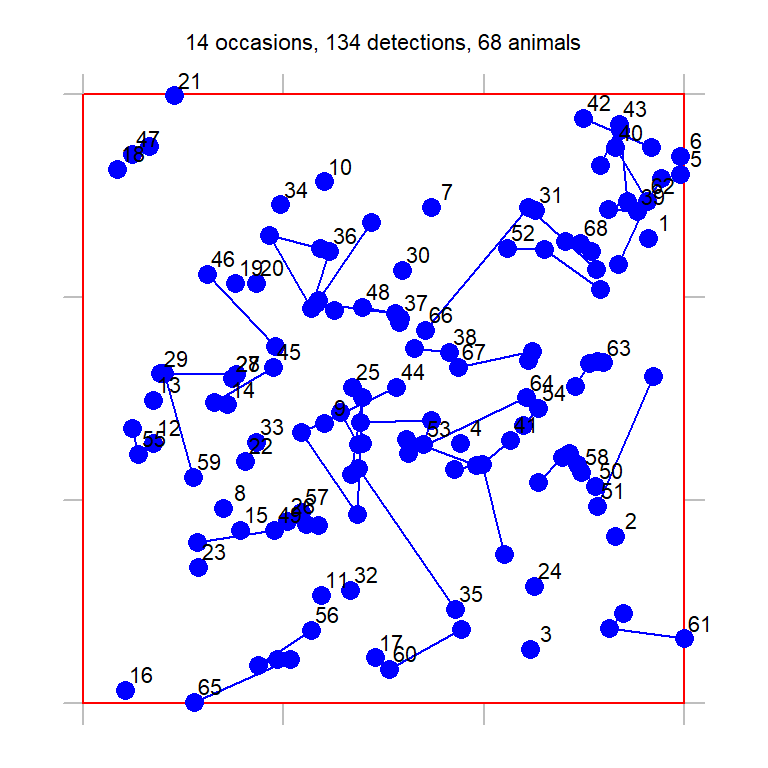
The ‘polygon’ detector type is used in secr for count data from searches of one or more areas (polygons). Transect detectors are the linear equivalent of polygons; as the theory and implementation are very similar we mostly refer to polygon detectors and only briefly mention transects. The relevant theory is in Chapter 4. The method may be used with individually identifiable cues (e.g., faeces) as well as for direct observations of individuals.

Cells of a polygon capthist contain the number of detections per animal per polygon per occasion, supplemented by the x-y coordinates of each detection).

Polygons may be independent (detector type ‘polygon’) or exclusive (detector type ‘polygonX’). Exclusivity is a particular type of dependence in which an animal may be detected at no more than one polygon on each occasion, resulting in binary data (i.e. polygons function more like multi-catch traps than ‘count’ detectors). Transect detectors also may be independent (‘transect’) or exclusive (‘transectX’).

D.1 Parameterisation

The detection model is fundamentally different for polygon detectors and detectors at a point (“single”, “multi”, “proximity”, “count”):

• For point detectors, the detection function directly models the probability of detection or the expected number of detections. All that matters is the distance between the animal’s centre and the detector.
• For polygon detectors, these quantities (probability or expected number) depend also on the geometrical relationships and the integration in Eq. 4.1. The detection function serves only to define the potential detections if the search area was unbounded (blue contours in Fig. 4.1).

We use a parameterisation that separates two aspects of detection – the expected number of cues from an individual (\lambda_c) and their spatial distribution given the animal’s location (h(\mathbf u| \mathbf x) normalised by dividing by H(\mathbf x) (Eq. 4.1). The parameters of h() are those of a typical detection function in secr (e.g., \lambda_0, \sigma), except that the factor \lambda_0 cancels out of the normalised expression. The expected number of cues, given an unbounded search area, is determined by a different parameter here labelled \lambda_c.

There are complications:

1. Rather than designate a new ‘real’ parameter lambdac, secr grabs the redundant intercept of the detection function (lambda0) and uses that for \lambda_c. Bear this in mind when reading output from polygon or transect models.

2. If each animal can be detected at most once per detector per occasion (as with exclusive detector types ‘polygonX’ and ‘transectX’) then instead of \lambda(\mathbf x) we require a probability of detection between 0 and 1, say g(\mathbf x). In secr the probability of detection is derived from the cumulative hazard using g(\mathbf x) = 1-\exp(-\lambda(\mathbf x)). The horned lizard dataset of Royle & Young (2008) has detector type ‘polygonX’ and their parameter ‘p’ was equivalent to 1 - \exp(-\lambda_c) (0 < p \le 1). For the same scenario and parameter Efford (2011) used p_\infty.

3. Unrelated to (2), detection functions in secr may model either the probability of detection (HN, HR, EX etc.) or the cumulative hazard of detection (HHN, HHR, HEX etc.) (see ?detectfn for a list). Although probability and cumulative hazard are mostly interchangeable for point detectors, it’s not so simple for polygon and transect detectors. The integration always uses the hazard form for h(\mathbf u | \mathbf x) (secr \ge 3.0.0)¹, and only hazard-based detection functions are allowed (HHN, HHR, HEX, HAN, HCG, HVP). The default function is HHN.

D.2 Example data: flat-tailed horned lizards

Royle & Young (2008) reported a Bayesian analysis of data from repeated searches for flat-tailed horned lizards (Phrynosoma mcallii) on a 9-ha square plot in Arizona, USA. Their dataset is included in secr as hornedlizardCH and will be used for demonstration. See ‘?hornedlizard’ for more details.

The lizards were free to move across the boundary of the plot and often buried themselves when approached. Half of the 134 different lizards were seen only once in 14 searches over 17 days. Fig. 2 shows the distribution of detections within the quadrat; lines connect successive detections of the individuals that were recaptured.

par(mar=c(1,1,2,1))
plot(hornedlizardCH, tracks = TRUE, varycol = FALSE, lab1cap = 
    TRUE, laboffset = 8, border = 10, title ='')

Locations of horned lizards on a 9-ha plot in Arizona (Royle & Young, 2008). Grid lines are 100 m apart.

D.3 Data input

Input of data for polygon and transect detectors is described in secr-datainput.pdf. It is little different to input of other data for secr. The key function is read.capthist, which reads text files containing the polygon or transect coordinates² and the capture records. Capture data should be in the ‘XY’ format of Density (one row per record with fields in the order Session, AnimalID, Occasion, X, Y). Capture records are automatically associated with polygons on the basis of X and Y (coordinates outside any polygon give an error). Transect data are also entered as X and Y coordinates and automatically associated with transect lines.

D.4 Fitting

The function secr.fit is used to fit polygon or transect models by maximum likelihood, exactly as for other detectors. Any model fitting requires a habitat mask – a representation of the region around the detectors possibly occupied by the detected animals (aka the ‘area of integration’ or ‘state space’). It’s simplest to use a simple buffer around the detectors, specified via the ‘buffer’ argument of secr.fit³. For the horned lizard dataset it is safe to use the default buffer width (100 m) and the default detection function (circular bivariate normal). We use trace = FALSE to suppress intermediate output that would be untidy here.

FTHL.fit <- secr.fit(hornedlizardCH, buffer = 80, trace = FALSE)
predict(FTHL.fit)

        link estimate SE.estimate      lcl      ucl
D        log  8.01307    1.061701  6.18740 10.37742
lambda0  log  0.13171    0.015128  0.10524  0.16485
sigma    log 18.50490    1.199388 16.29950 21.00871

The estimated density is 8.01 / ha, somewhat less than the value given by Royle & Young (2008); see Efford (2011) for an explanation, also Marques et al. (2011) and Dorazio (2013). The parameter labelled ‘lambda0’ (i.e. \lambda_c) is equivalent to p in Royle & Young (2008) (using \hat p \approx 1 - \exp(-\hat \lambda_c)).

FTHL.fit is an object of class ‘secr’. We would use the ‘plot’ method to graph the fitted detection function :

plot(FTHL.fit, xv = 0:70, ylab = 'p')

D.5 Cue data

By ‘cue’ in this context we mean a discrete sign identifiable to an individual animal by means such as microsatellite DNA. Faeces and passive hair samples may be cues. Animals may produce more than one cue per occasion. The number of cues in a specific polygon then has a discrete distribution such as Poisson, binomial or negative binomial.

A cue dataset is not readily available, so we simulate some cue data to demonstrate the analysis. The text file ‘polygonexample1.txt’ contains the boundary coordinates.

datadir <- system.file("extdata", package = "secr")
file1 <- paste0(datadir, '/polygonexample1.txt')
example1 <- read.traps(file = file1, detector = 'polygon')
polygonCH <- sim.capthist(example1, popn = list(D = 1, 
    buffer = 200), detectfn = 'HHN', detectpar = list(
    lambda0 = 5, sigma = 50), noccasions = 1, seed = 123)

par(mar = c(1,2,3,2))
plot(polygonCH, tracks = TRUE, varycol = FALSE, lab1cap = TRUE,
    laboffset = 15, title = paste("Simulated 'polygon' data", 
    "D = 1, lambda0 = 5, sigma = 50"))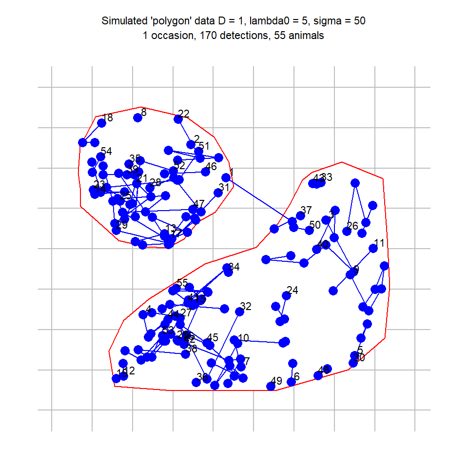

Figure D.1: Simulated cue data from a single search of two irregular polygons.

Our simulated sampling was a single search (noccasions = 1), and the intercept of the detection function (lambda0 = 5) is the expected number of cues that would be found per animal if the search was unbounded. The plot (Fig. D.1) is slightly misleading because, although ‘tracks = TRUE’ serves to link cues from the same animal, the cues are not ordered in time.

To fit the model by maximum likelihood we use secr.fit as before:

cuesim.fit <- secr.fit(polygonCH, buffer = 200, trace = FALSE)
predict(cuesim.fit)

        link estimate SE.estimate      lcl     ucl
D        log   1.1035     0.15366  0.84099  1.4478
lambda0  log   4.3764     0.41885  3.62938  5.2771
sigma    log  49.4464     2.43133 44.90613 54.4457

D.6 Discretizing polygon data

An alternative way to handle polygon capthist data is to convert it to a raster representation i.e. to replace each polygon with a set of point detectors, each located at the centre of a square pixel. Point detectors (‘multi’, ‘proximity’, ‘count’ etc.) tend to be more robust and models often fit faster. They also allow habitat attributes to be associated with detectors at the scale of a pixel rather than the whole polygon. The secr function discretize performs the necessary conversion in a single step. Selection of an appropriate pixel size (spacing) is up to the user. There is a tradeoff between faster execution (larger pixels are better) and controlling artefacts from the discretization, which can be checked by comparing estimates with different levels of spacing.

Taking our example from before,

discreteCH <- discretize (polygonCH, spacing = 20)
par(mar = c(1,2,3,2))
plot(discreteCH, varycol = FALSE, tracks = TRUE)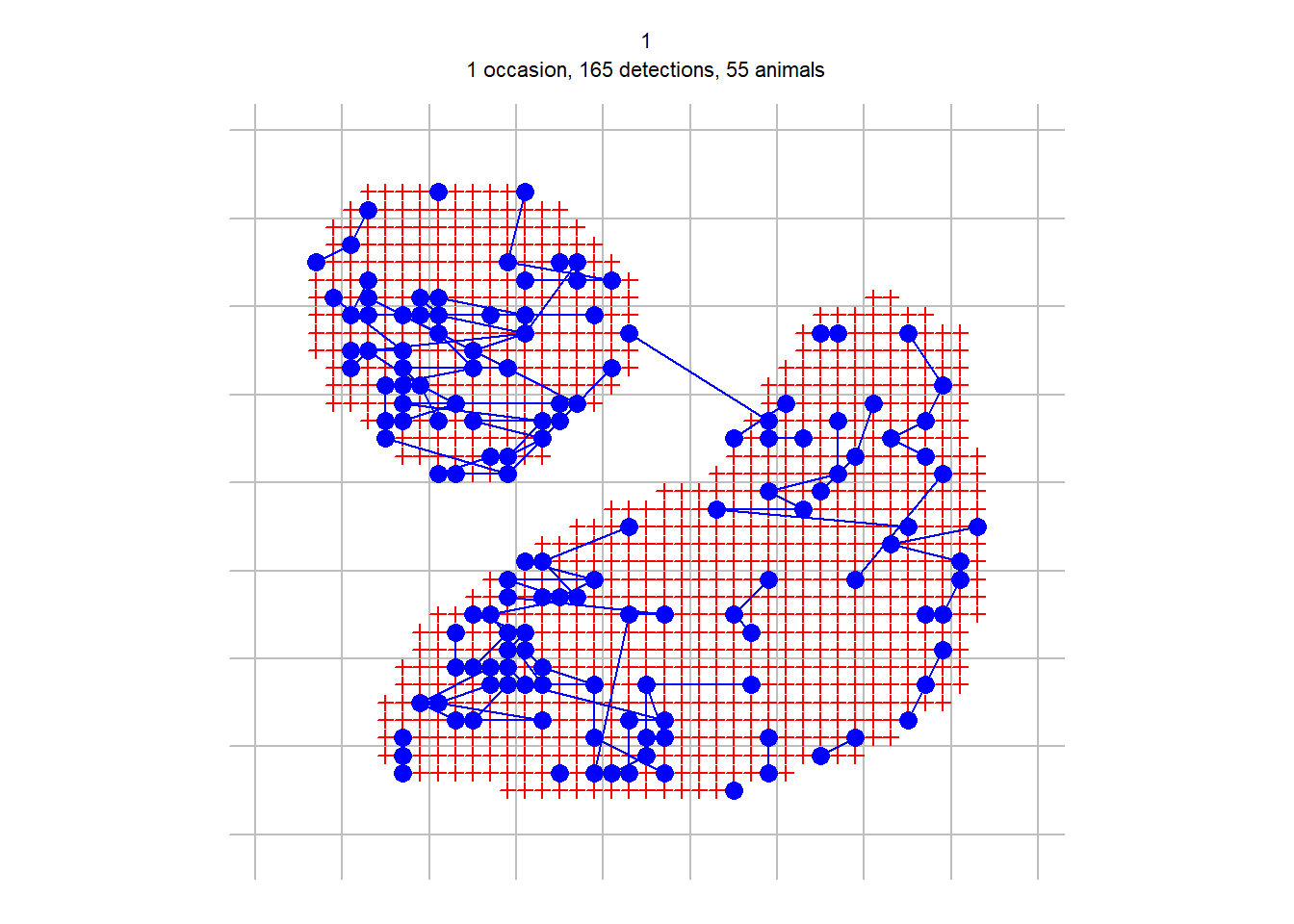

Discretized area search data

discrete.fit <- secr.fit(discreteCH, buffer = 200, detectfn = 
    'HHN', trace = FALSE)
predict(discrete.fit)

        link estimate SE.estimate       lcl      ucl
D        log  1.09535    0.152768  0.834463  1.43780
lambda0  log  0.11205    0.014492  0.087048  0.14422
sigma    log 49.83842    2.673999 44.867021 55.36066

Post-hoc discretization is also considered by Russell et al. (2012), Milleret et al. (2018) and Paterson et al. (2019).

D.7 Transect search

Transect data, as understood here, include the positions from which individuals are detected along a linear route through 2-dimensional habitat. They do not include distances from the route to the location of the individual, at least, not yet. A route may be searched multiple times, and a dataset may include multiple routes, but neither of these is necessary. Searches of linear habitat such as river banks require a different approach - see the package secrlinear.

We simulate some data for an imaginary wiggly transect.

x <- seq(0, 4*pi, length = 20)
transect <- make.transect(x = x*100, y = sin(x)*300, 
    exclusive = FALSE)
summary(transect)

Object class       traps 
Detector type      transect 
Number vertices    20 
Number transects   1 
Total length       2756.1 m 
x-range            0 1256.6 m 
y-range            -298.98 298.98 m 

transectCH <- sim.capthist(transect, popn = list(D = 2, 
    buffer = 300), detectfn = 'HHN', detectpar = list(
    lambda0 = 1.0, sigma = 50), binomN = 0, seed = 123)

By setting exclusive = FALSE we signal that there may be more than one detection per animal per occasion on this single transect (i.e. this is a ‘transect’ detector rather than ‘transectX’).

Constructing a habitat mask explicitly with make.mask (rather than relying on ‘buffer’ in secr.fit) allows us to specify the point spacing and discard outlying points (Fig. D.2).

transectmask <- make.mask(transect, type = 'trapbuffer', buffer = 300, spacing = 20)
par(mar = c(3,1,3,1))
plot(transectmask, border = 0)
plot(transect, add = TRUE, detpar = list(lwd = 2))
plot(transectCH, tracks = TRUE, add = TRUE, title = '')

Figure D.2: Habitat mask (grey dots) and simulated transect data from five searches of a 2.8-km transect. Colours differ between individuals, but are not unique.

Model fitting uses secr.fit as before. We specify the distribution of the number of detections per individual per occasion as Poisson (binomN = 0), although this also happens to be the default. Setting method = ‘Nelder-Mead’ is slightly more likely to yield valid estimates of standard errors than using the default method (see Technical notes).

transect.fit <- secr.fit(transectCH, mask = transectmask, 
    binomN = 0, method = 'Nelder-Mead', trace = FALSE)

Occasional ‘ier’ error codes may be ignored (see Technical notes). The estimates are close to the true values except for sigma, which may be positively biased.

predict (transect.fit)

        link estimate SE.estimate      lcl     ucl
D        log   1.8527    0.196674  1.50552  2.2798
lambda0  log   1.0415    0.080433  0.89539  1.2114
sigma    log  53.6290    2.313387 49.28317 58.3581

Another way to analyse transect data is to discretize it. We divide the transect into 25-m segments and then change the detector type. In the resulting capthist object the transect has been replaced by a series of proximity detectors, each at the midpoint of a segment.

snippedCH <- snip(transectCH, by = 25)
snippedCH <- reduce(snippedCH, outputdetector = 'proximity')

The same may be achieved with newCH <- discretize(transectCH, spacing = 25). We can fit a model using the same mask as before. The result differs in the scaling of the lambda0 parameter, but in other respects is similar to that from the transect model.

snipped.fit <- secr.fit(snippedCH, mask = transectmask, 
    detectfn = 'HHN', trace = FALSE)
predict(snipped.fit)

        link estimate SE.estimate      lcl      ucl
D        log  1.84217    0.195625  1.49689  2.26708
lambda0  log  0.19312    0.018034  0.16089  0.23182
sigma    log 53.67901    2.321128 49.31908 58.42436

D.8 More on polygons

The implementation in secr allows any number of disjunct polygons or non-intersecting transects.

Polygons may be irregularly shaped, but there are some limitations in the default implementation. Polygons may not be concave in an east-west direction, in the sense that there are more than two intersections with a vertical line. Sometimes east-west concavity may be fixed by rotating the polygon and its associated data points (see function rotate). Polygons should not contain holes, and the polygons used on any one occasion should not overlap.

The polygon on the left is not allowed because its boundary is intersected by a vertical line at more than two points.

D.8.1 Solutions for non-conforming polygons

1. Break into parts

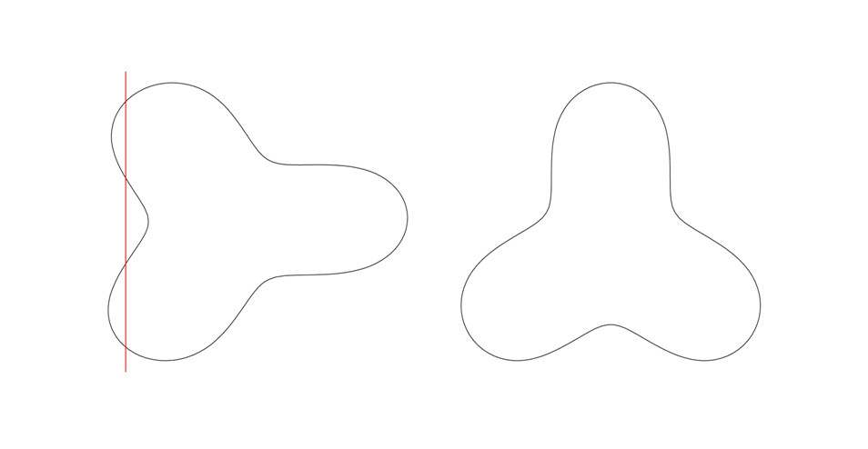
One solution to ‘east-west concavity’ is to break the offending polygon into two or more parts. For this you need to know which vertices belong in which part, but that is (usually) easily determined from a plot. In this real example we recognise vertices 11 and 23 as critical, and split the polygon there. Note the need to include the clip vertices in both polygons, and to maintain the order of vertices. Both example2 and newpoly are traps objects.

file2 <- paste0(datadir, '/polygonexample2.txt')
example2 <- read.traps(file = file2, detector = 'polygon')
par(mfrow = c(1,2), mar = c(2,1,1,1))
plot(example2)
text(example2$x, example2$y, 1:nrow(example2), cex = 0.7)
newpoly <- make.poly (list(p1 = example2[11:23,], 
  p2 = example2[c(1:11, 23:27),]))

No errors found :-)

plot(newpoly, label = TRUE)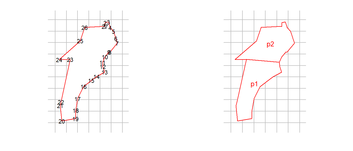

Splitting a non-conforming polygon

Attributes such as covariates and usage must be rebuilt by hand.

2. Pointwise testing

Another solution is to evaluate whether each point chosen dynamically by the integration code lies inside the polygon of interest. This is inevitably slower than the default algorithm that assumes all points between the lower and upper intersections lie within the polygon. Select the slower, more general option by setting details = list(convexpolygon = FALSE).

D.9 Technical notes

Fitting models for polygon detectors with secr.fit requires the hazard function to be integrated in two-dimensions many times. In secr >= 4.4 this is done with repeated one-dimensional Gaussian quadrature using the C++ function ‘integrate’ in RcppNumerical (Qiu et al., 2023).

Polygon and transect SECR models seem to be prone to numerical problems in estimating the information matrix (negative Hessian), which flow on into poor variance estimates and missing values for the standard errors of ‘real’ parameters. At the time of writing these seem to be overcome by overriding the default maximization method (Newton-Raphson in ‘nlm’) and using, for example, “method = ‘BFGS’”. Another solution, perhaps more reliable, is to compute the information matrix independently by setting ‘details = list(hessian = ’fdhess’)’ in the call to secr.fit. Yet another approach is to apply secr.refit with “method = ‘none’” to a previously fitted model to compute the variances.

The algorithm for finding a starting point in parameter space for the numerical maximization is not entirely reliable; it may be necessary to specify the ‘start’ argument of secr.fit manually, remembering that the values should be on the link scale (default log for D, lambda0 and sigma).

Data for polygons and transects are unlike those from detectors such as traps in several respects:

• The association between vertices in a ‘traps’ object and polygons or transects resides in an attribute ‘polyID’ that is out of sight, but may be retrieved with the polyID or transectID functions. If the attribute is NULL, all vertices are assumed to belong to one polygon or transect.

• The x-y coordinates for each detection are stored in the attribute ‘detectedXY’ of a capthist object. To retrieve these coordinates use the function xy. Detections are ordered by occasion, animal, and detector (i.e., polyID).

• subset or split applied to a polygon or transect ‘traps’ object operate at the level of whole polygons or transects, not vertices (rows).

• usage also applies to whole polygons or transects. The option of specifying varying usage by occasion is not fully tested for these detector types.

• The interpretation of detection functions and their parameters is subtly different; the detection function must be integrated over 1-D or 2-D rather than yielding a probability directly (see Efford (2011)).

Dorazio, R. M. (2013). Bayes and empirical bayes estimators of abundance and density from spatial capture-recapture data. PLoS ONE, 8, e84017.

Efford, M. G. (2011). Estimation of population density by spatially explicit capture-recapture analysis of data from area searches. Ecology, 92, 2202–2207.

Kendeigh, S. C. (1944). Measurement of bird populations. Ecological Monographs, 14, 67–106. https://doi.org/10.2307/1961632

Marques, T. A., Thomas, L., & Royle, J. A. (2011). A hierarchical model for spatial capture-recapture data: comment. Ecology, 92, 526–528.

Milleret, C., Dupont, P., Brøseth, H., Kindberg, J., Royle, J. A., & Bischof, R. (2018). Using partial aggregation in spatial capture recapture. Methods in Ecology and Evolution, 9(8), 1896–1907. https://doi.org/10.1111/2041-210x.13030

Paterson, J. T., Proffitt, K., Jimenez, B., Rotella, J., & Garrott, R. (2019). Simulation-based validation of spatial capture-recapture models: A case study using mountain lions. PLOS ONE, 14(4), e0215458. https://doi.org/10.1371/journal.pone.0215458

Qiu, Y., Balan, S., Beall, M., Sauder, M., Okazaki, N., & Hahn, T. (2023). RcppNumerical: ’Rcpp’ integration for numerical computing libraries. https://CRAN.R-project.org/package=RcppNumerical

Royle, J. A., & Young, K. V. (2008). A hierarchical model for spatial capture-recapture data. Ecology, 89, 2281–2289.

Russell, R. E., Royle, J. A., Desimone, R., Schwartz, M. K., Edwards, V. L., Pilgrim, K. P., & Mckelvey, K. S. (2012). Estimating abundance of mountain lions from unstructured spatial sampling. The Journal of Wildlife Management, 76(8), 1551–1561. https://doi.org/10.1002/jwmg.412

---

1. The logic here is that hazards are additive whereas probabilities are not.

2. For constraints on the shape of polygon detectors see Polygon shape

3. Alternatively, one can construct a mask with make.mask and provide that in the ‘mask’ argument of secr.fit. Note that make.mask defaults to type = 'rectangular'; see Transect search for an example in which points are dropped if they are within the rectangle but far from detectors (the default in secr.fit)