fit <- secr.fit(hareCH6, buffer = 250, CL = FALSE, trace = FALSE) # default
fitCL <- secr.fit(hareCH6, buffer = 250, CL = TRUE, trace = FALSE)Appendix B — Faster is better
There is nothing virtuous about waiting days for a model to fit if there is a faster alternative. Here are some things you can do.
B.1 Mask tuning
Consider carefully the necessary extent of your habitat mask and the acceptable cell size (Chapter 12 has detailed advice). If your detectors are clustered then your mask may have gaps between the clusters (use type = ‘trapbuffer’ in make.mask). Masks with more than 2000 points are generally excessive (and the default is about 4000!).
B.2 Conditional likelihood
The default in secr.fit is to maximize the full likelihood (i.e., to jointly fit both the state process and the observation process). If you do not need to model spatial, temporal or group-specific variation in density (the sole real parameter of the state model) then you can save time by first fitting only the observation process. This is achieved by maximizing only the likelihood conditional on n, the number of detected individuals (Borchers & Efford, 2008). Conditional likelihood maximization is selected in secr.fit by setting CL = TRUE.
Selecting an observation model with CL = TRUE (and first focussing on detection parameters) is a good strategy even if you intend to model density later. It may occasionally be desirable to re-visit the selection if covariates can affect both density and detection parameters.
Fitting time is reduced by 43% because maximization is over two parameters (g0, sigma) instead of three. The relative reduction will be less for more complex detection models, but still worthwhile.
Having selected a suitable observation model with CL = TRUE you can then either resort to a full-likelihood fit to estimate density, or compute a Horvitz-Thompson-like (HT) estimate in function derived. In models without individual covariates the HT estimate is n/a(\hat \theta) where n is the number of detected individuals, \theta represents the parameters of the observation model, and a is the effective sampling area as a function of the estimated detection parameters.
Compare
predict(fit) # CL = FALSE link estimate SE.estimate lcl ucl
D log 1.465987 0.1913125 1.136361 1.891228
g0 logit 0.061584 0.0093004 0.045686 0.082536
sigma log 68.345777 4.4693114 60.132427 77.680970derived(fitCL) # CL = TRUE estimate SE.estimate lcl ucl CVn CVa CVD
esa 46.385 NA NA NA NA NA NA
D 1.466 0.19051 1.1376 1.8892 0.12127 0.046715 0.12995Estimated density is exactly the same, to 6 significant figures (1.46599). This is expected when n is Poisson; slight differences arise when n is binomial (because the number of animals N in the masked area is considered fixed rather than random). The estimated variance differs slightly - that from derived follows an unpublished and slightly ad hoc procedure (Borchers & Efford, 2007).
B.3 Mashing
Mashing is a very effective way of speeding up estimation when the design uses many replicate clusters of detectors, each with the same geometry, and clusters are far enough apart that animals are not detected on more than one. The approach for M clusters is to overlay all data as if from a single cluster; the estimated density will be M times the per-cluster estimate, and SE etc. will be inflated by the same factor. This relies on individuals being detected independently of each other, which is a standard assumption in any case. The present implementation assumes density is uniform.
The capthist object is first collapsed with function mash into one using the geometry of a single cluster. The object retains a memory of the number of individuals from each original cluster in the attribute ‘n.mash’. Functions derived, derivedMash and the method predict.secr use ‘n.mash’ to adjust their output density, SE, and confidence limits.
We describe in general terms an actual example in which 18 separated clusters of 12 traps were operated on 6 occasions. Each cluster had the same geometry (two parallel rows of traps separated by 200 m along and between rows). Trap numbering was consistently up one row and down the other. The capthist object CH included detections of 150 animals in the 216 traps. To mash these data we first assign attributes for the cluster number (clusterID) and the sequence number of each trap within its cluster (clustertrap). The function mash then collapses the data as if all detections were made on one cluster. A mask based on this single notional cluster has many fewer points than a mask with the same spacing spanning all clusters.
The model for the mashed data fitted in 4% of the time required for the original. The mashed estimate of density shrank by 2% in this case, which is probably due to slight variation among clusters in the actual spacing of traps (one cluster was arbitrarily chosen to represent all clusters). Mashing prevents the inclusion of cluster-specific detail in the model (such as discontinuous habitat near the traps). For further details see ?mash.
B.4 Parallel fitting
Your computer almost certainly has multiple cores, allowing computations to run in parallel.
Multi-threading in secr.fit uses multiple cores. By default only 2 cores are used (a limit set by CRAN), and this should almost certainly be increased. The number of threads is set with setNumThreads() or the ‘ncores’ argument. The marginal benefit of increasing the number of threads declines as more are added. Modify the following benchmark code for your own example. For models that are very slow to fit, relative values may be got more quickly by performing a single likelihood evaluation with secr.fit(..., details = list(LLonly = TRUE)).
code for benchmark timing
library(microbenchmark)   # install this package first
cores <- c(2,4,6,8)
jobs <- lapply(cores, function(nc) {
    bquote(suppressWarnings(
        secr.fit(captdata, trace = FALSE, ncores = .(nc))
    ))})
names(jobs) <- paste("ncores = ", cores)
microbenchmark(list = jobs, times = 10, unit = "seconds")
Unit: seconds
expr min lq mean median uq max neval
ncores = 2 2.03325 2.08653 2.56186 2.31389 3.1715 3.2989 10
ncores = 4 1.09336 1.21461 1.45341 1.33114 1.7241 1.8581 10
ncores = 6 0.86954 1.02736 1.10523 1.06195 1.1171 1.6480 10
ncores = 8 0.81599 0.83314 0.98474 0.96208 1.0265 1.3466 10See ?Parallel for more.
B.5 Reducing complexity (session- or group-specific models)
Simultaneous estimation of many parameters can be painfully slow, but it can be completely avoided. If your model is fully session- or group-specific then it is much faster to analyse each group separately. For sessions this is can be done simply with lapply (Section 14.6). For groups you may need to construct new capthist objects using subset to extract groups corresponding to the levels of one or more individual covariates.
B.6 Reducing number of levels of detection covariates
secr.fit pre-computes a lookup table of values for detection parameters. The size of the table increases with the number of unique levels of any covariates. A continuous individual or detector covariate can have many similar levels. Binning covariate values can give a large saving in memory and time (see ?binCovariate).
B.7 Collapsing occasions
If there is no temporal aspect to the model you want to fit (such as a behavioural response) and detectors are independent (not true for traps i.e. “multi”) then it is attractive to collapse all sampling occasions. This happens automatically by default for ‘proximity’ and ‘count’ detectors (details argument ‘fastproximity = TRUE’). For example, with the Tennessee black bear data we get:
code to compare fastproximity on/off
# Great Smoky Mountains black bear hair snag data
# Deliberately slow both fits down by setting ncores = 2
old <- setNumThreads(2)

# mask using park boundary GSM
msk <- make.mask(traps(blackbearCH), buffer = 6000, type = 'trapbuffer',
                 poly = GSM, keep.poly = FALSE)

# 'fastproximity' On (default for 'proximity' detectors)
bbfitfaston <- secr.fit(blackbearCH, mask = msk, trace = FALSE)

# 'fastproximity' Off
bbfitfastoff <- secr.fit(blackbearCH, mask = msk, trace = FALSE,
                      details = list(fastproximity = FALSE))

# summary
fits <- secrlist(bbfitfaston, bbfitfastoff)

cat("Compare density estimates\n")
collate(fits)[,,,'D']
cat ("\nCompare timing\n")
sapply(fits, '[[', 'proctime')
Compare density estimates
estimate SE.estimate lcl ucl
bbfitfaston 0.0084355 0.00081891 0.006977 0.010199
bbfitfastoff 0.0084355 0.00081890 0.006977 0.010199
Compare timing
bbfitfaston.elapsed bbfitfastoff.elapsed
3.97 13.82 Data may be collapsed in reduce.capthist without loss of data by choosing ‘outputdetector’ carefully and setting by = “ALL”. The collapsed capthist object receives a usage attribute equal to the sum of occasion-specific usages. In this case usage is the number of collapsed occasions (10) and the collapsed model fits a Binomial probability with size = 10 rather than a Bernoulli probability per occasion.
B.8 Individual mask subsets
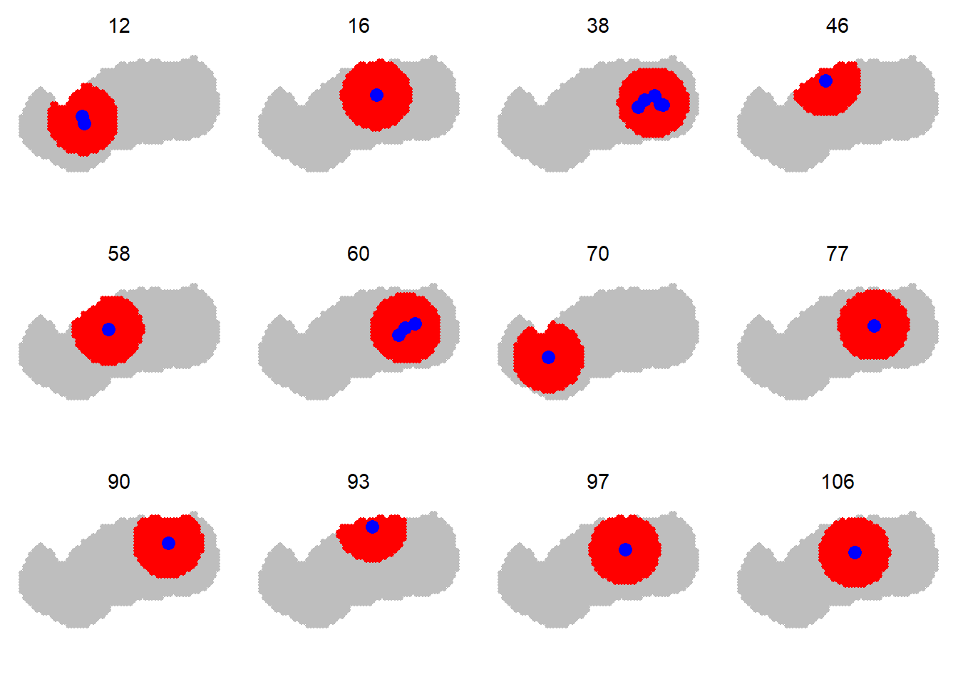
secr allows the user to customise the mask for each detected animal by considering only a subset of points. The subset is defined by a radius in metres around the centroid of detections; set this using the details argument ‘maxdistance’. Speed gains vary with the layout, but can exceed 2-fold. Bias results when the radius is too small (try 5\sigma or the buffer distance).
Here we extend the preceding black bear example. The mask used for each bear is restricted to points within 6 km of the centroid of its detections. There is a >2\times speed gain without significant change in the density estimates.
code to plot sample of individual masks
centr <- centroids(blackbearCH)
par(mfrow=c(3,4), mar=c(1,1,1,1))
for (i in sort(sample.int(139, size=12))) {
    plot(msk, border = 10)
    plot(subset(msk, distancetotrap(msk, centr[i,])<6000), add = TRUE,
         col = 'red')
    plot(subset(blackbearCH, i), varycol = FALSE, add = TRUE, title = '',
         subtitle = '')
    mtext(side = 3, i, line = -1, cex = 0.9 )
}
code to compare individual mask subsets
old <- setNumThreads(2)
# fastproximity default
bbfitfaston <- secr.fit(blackbearCH, mask = msk, trace = FALSE)
bbfitfastonmaxd <- secr.fit(blackbearCH, mask = msk, trace = FALSE,
                      details = list(maxdistance = 6000))

fits <- secrlist(bbfitfaston, bbfitfastonmaxd)

cat("Compare density estimates\n")
collate(fits)[,,,'D']
cat ("\nCompare timing\n")
sapply(fits, '[[', 'proctime')
Compare density estimates
estimate SE.estimate lcl ucl
bbfitfaston 0.0084355 0.00081891 0.0069770 0.010199
bbfitfastonmaxd 0.0084421 0.00081855 0.0069841 0.010204
Compare timing
bbfitfaston.elapsed bbfitfastonmaxd.elapsed
4.00 1.33 B.9 Collapsing detectors
The benefit from collapsing occasions has a spatial analogue: if there are many detectors and they are closely spaced relative to animal movements \sigma then nearby detectors may be aggregated into new notional detectors located at the centroid. The reduce.traps method has an argument ‘span’ explained as follows in the help –
If ‘span’ is specified a clustering of detector sites will be performed with
hclustand detectors will be assigned to groups withcutree. The default algorithm inhclustis complete linkage, which tends to yield compact, circular clusters; each will have diameter less than or equal to ‘span’.
B.10 “multi” detector type instead of “proximity”
The type of the detectors is usually determined by the sampling reality. For example, if individuals can physically be detected at several sites on one occasion then the “proximity” detector type is preferred over “multi”. However, if data are very sparse, so that individuals in practice are almost never observed at multiple sites on one occasion, then the detectors may as well be of type “multi”, in the sense that there is no observable difference between the two types of detection process. “multi” models used to fit much more quickly than “proximity” models, and this is still true for elaborate or time-dependent models that cannot use the ‘fastproximity’ option.
B.11 Some models are just slower than others
Detector covariates pose a particular problem. Models with learned responses take slightly longer to fit.