datadir <- system.file("extdata", package = "secr")
OVforest <- sf::st_read (paste0(datadir, "/OVforest.shp"),
    quiet = TRUE)
# drop points we don't need
leftbank <- read.table(paste0(datadir,"/leftbank.txt"))[21:195,]
options(digits = 6, width = 95) 11 Density model
Spatially explicit capture–recapture models allow for population density to vary over space (Borchers & Efford, 2008). Density is the intensity of a spatial Poisson process for activity centres. Models for density may include spatial covariates (e.g., vegetation type, elevation) and spatial trend.
In Chapter 10 we introduced linear sub-models for detection parameters. Here we consider SECR models in which the population density at any point, considered on the link scale, is also a linear function of V covariates1. For density this means
\begin{equation} D(\mathbf x; \phi) = f^{-1}[\phi_0 + \sum_{v=1}^V c_v(\mathbf x) \, \phi_v], \end{equation} where c_v(\mathbf x) is the value of the v-th covariate at point \mathbf x, \phi_0 is the intercept, \phi_v is the coefficient for the v-th covariate, and f^{-1} is the inverse of the link function. Commonly we model the logarithm of density and f^{-1} is the exponential function.
Although D(\mathbf x;\phi) is often a smooth function, in secr we evaluate it only at the fixed points of the habitat mask (Chapter 12). A mask defines the region of habitat relevant to a particular study: in the simplest case it is a buffered zone inclusive of the detector locations. More complex masks may exclude interior areas of non-habitat or have an irregular outline.
A density model D(\mathbf x;\phi) is specified in the ‘model’ argument of secr.fit2. Spatial covariates, if any, are needed for each mask point; they are stored in the ‘covariates’ attribute of the mask. Results from fitting the model (including the estimated coefficients \phi) are saved in an object of class ‘secr’. To visualise a fitted density model we first evaluate it at each point on a mask with the function predictDsurface. This creates an object of class ‘Dsurface’. A Dsurface is a mask with added density data, and plotting a Dsurface is like plotting a mask covariate.
secr.fit.
| Formula | Effect |
|---|---|
| D \sim cover | density varies with ‘cover’, a variable in covariates(mask) |
| list(D \sim g, g0 \sim g) | both density and g0 differ between groups |
| D \sim session | session-specific density |
11.1 Absolute vs relative density
The conventional approach to density surfaces is to fit a model of absolute density by maximizing the ‘full’ likelihood. Until recently, maximizing the likelihood conditional on n, the number detected, was thought to work only when density was assumed to be uniform (homogeneous), placing it outside the scope of this chapter. However, recent extensions to secr allow models of relative density to be fitted by maximizing the conditional likelihood (CL = TRUE in secr.fit), and this has some advantages (Efford, 2025). Relative density differs from absolute density by a constant factor. This chapter stresses modelling absolute density and keeps relative density for a section at the end.
11.2 Brushtail possum example
For illustration we use a brushtail possum (Trichosurus vulpecula) dataset from the Orongorongo Valley, New Zealand. Possums were live-trapped in mixed evergreen forest near Wellington for nearly 40 years (Efford & Cowan, 2004). Single-catch traps were set for 5 consecutive nights, three times a year. The dataset ‘OVpossumCH’ has data from the years 1996 and 1997. The study grid was bounded by a shingle riverbed to the north and west. See ?OVpossum in secr for more details.
First we import data for the habitat mask from a polygon shapefile included with the package:
OVforest is now a simple features (sf) object defined in package sf. We build a habitat mask object, selecting the first two polygons in OVforest and discarding the third that lies across the river. The attribute table of the shapefile (and hence OVforest) includes a categorical variable ‘forest’ that is either ‘beech’ (Nothofagus spp.) or ‘nonbeech’ (mixed podocarp-hardwood); addCovariates attaches these data to each cell in the mask.
ovtrap <- traps(OVpossumCH[[1]])
ovmask <- make.mask(ovtrap, buffer = 120, type = "trapbuffer",
    poly = OVforest[1:2,], spacing = 7.5, keep.poly = FALSE)
ovmask <- addCovariates(ovmask, OVforest[1:2,])
Plotting is easy:
code to plot possum mask
par(mar = c(1,6,2,8))
forestcol <- terrain.colors(6)[c(4,2)]
plot(ovmask, cov="forest", dots = FALSE, col = forestcol)
plot(ovtrap, add = TRUE)
par(cex = 0.8)
terra::sbar(d = 200, xy = c(2674670, 5982930), type = 'line',
    divs = 2, below = "metres", labels = c("0","100","200"),
    ticks = 10)
terra::north(xy = c(2674670, 5982830), d = 40, label = "N")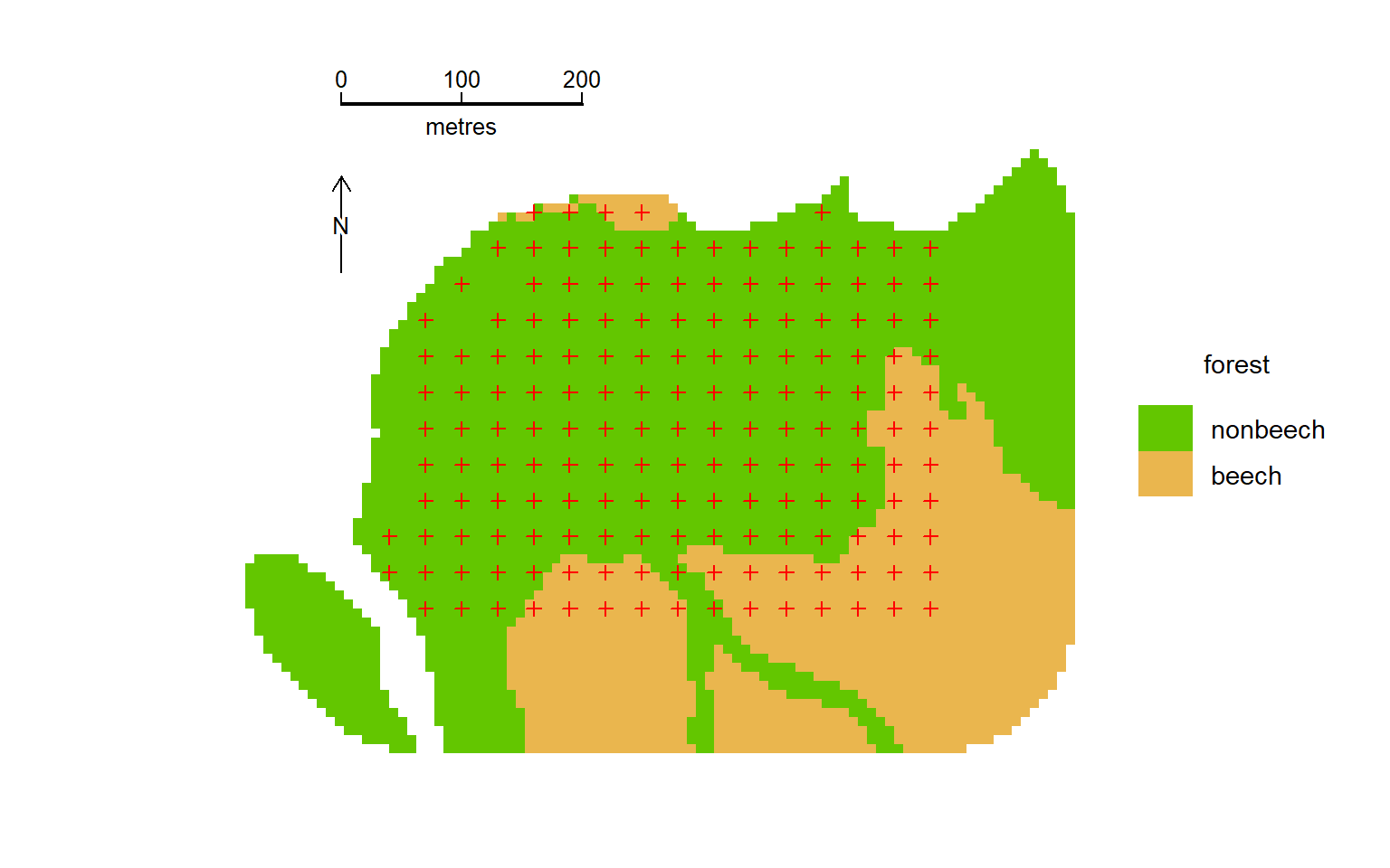
We next fit some simple models to data from February 1996 (session 49). Some warnings are suppressed for clarity.
        npar   logLik  dAIC  AICwt
Dxy2       8 -1549.32 0.000 0.4429
Dxy        5 -1552.86 1.086 0.2573
Dforest    4 -1554.15 1.653 0.1938
null       3 -1555.75 2.860 0.1060
Each of the inhomogeneous models seems marginally better than the null model, but there is little to choose among them.
To visualise the entire surface we compute predicted density at each mask point. For example, we can plot the quadratic surface like this:
par(mar = c(1,6,2,8))
surfaceDxy2 <- predictDsurface(fits$Dxy2)
plot(surfaceDxy2, plottype = "shaded", poly = FALSE, breaks =
      seq(0,22,2), title = "Density / ha", text.cex = 1)
# graphical elements to be added, including contours of Dsurface
plot(ovtrap, add = TRUE)
plot(surfaceDxy2, plottype = "contour", poly = FALSE, breaks =
    seq(0,22,2), add = TRUE)
lines(leftbank)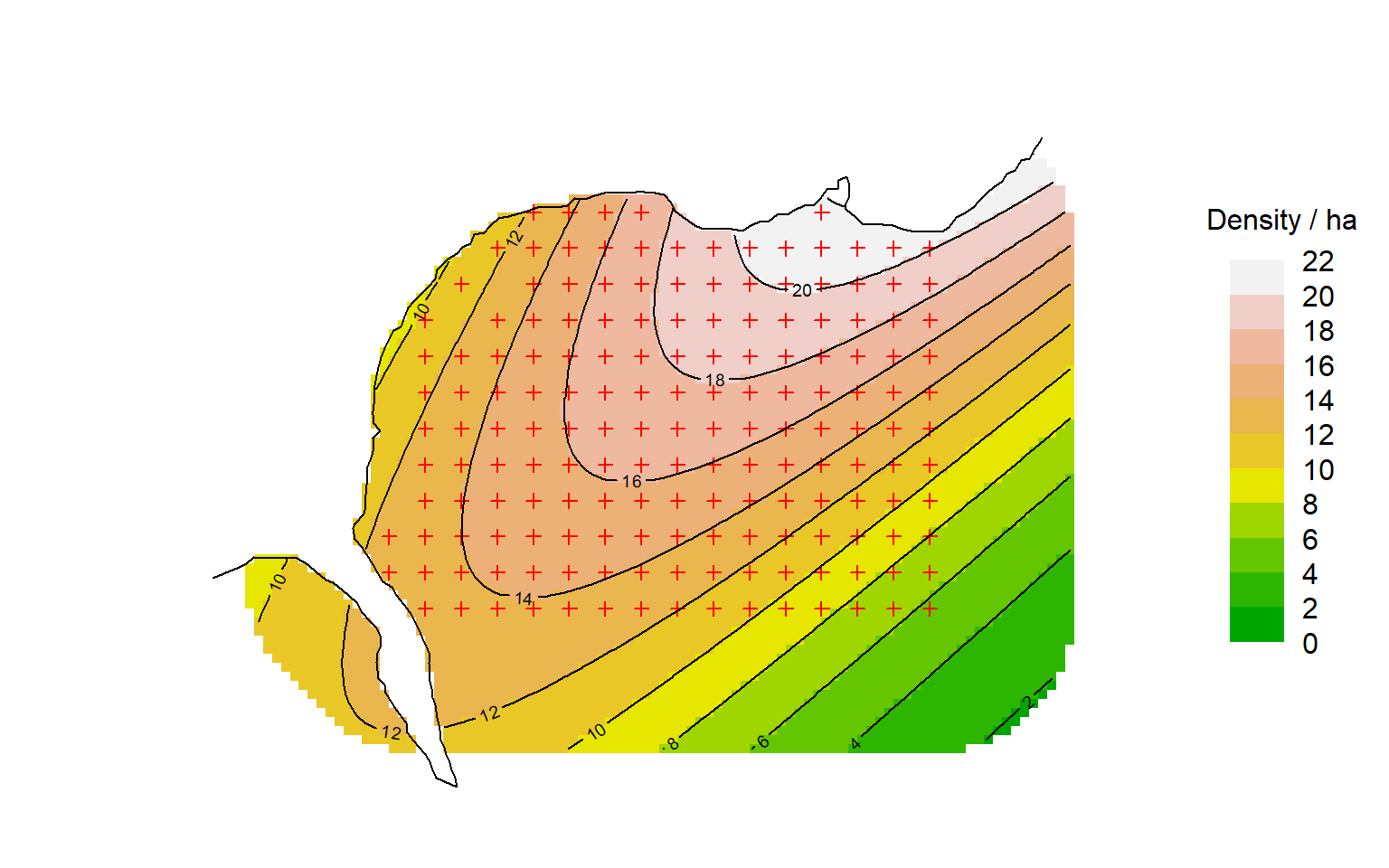
Following sections expand on the options for specifying and displaying density models.
11.3 Using the ‘model’ argument
A model formula defines variation in each parameter as a function of covariates (including geographic coordinates and their polynomial terms) that is linear on the ‘link’ scale, as in a generalized linear model.
The options differ between the state and observation models. D may vary with respect to group, session or point in space
The predictors ‘group’ and ‘session’ behave for D as they do for other real parameters. They determine variation in the expected density for each group or session that is (by default) uniform across space, leading to a homogeneous Poisson model and a flat surface. No further explanation is therefore needed.
11.3.1 Link function
The default link for D is ‘log’. It is equally feasible in most cases to choose ‘identity’ as the link (see the secr.fit argument ‘link’), and for the null model D \sim 1 the estimate will be the same to numerical accuracy, as will estimates involving only categorical variables (e.g., session). However, with an ‘identity’ link the usual (asymptotic) confidence limits will be symmetrical (unless truncated at zero) rather than asymmetrical. In models with continuous predictors, including spatial trend surfaces, the link function will affect the result, although the difference may be small when the amplitude of variation on the surface is small. Otherwise, serious thought is needed regarding which model is biologically more appropriate: logarithmic or linear.
The ‘identity’ link may cause problems when density is very small or very large because, by default, the maximization method assumes all parameters have similar scale (e.g., typsize = c(1,1,1) for default constant models). Setting typsize manually in a call to secr.fit can fix the problem and speed up fitting. For example, if density is around 0.001/ha (10 per 100 km^2) then call secr.fit(..., typsize = c(0.001,1,1)) (typsize has one element for each beta parameter). Problems with the identity link mostly disappear when modelling relative density (CL = TRUE) because coefficients are automatically scaled by the intercept. See Appendix I for more on link functions.
You may wonder why secr.fit is ambivalent regarding the link function: link functions have seemed a necessary part of the machinery for capture–recapture modelling since Lebreton et al. (1992). Their key role is to keep the ‘real’ parameter within feasible bounds (e.g., 0-1 for probabilities). In secr.fit any modelled value of D that falls below zero is truncated at zero (of course this condition will not arise with a log link).
11.3.2 Built-in variables
secr.fit automatically recognises the spatial variables x, y, x2, y2 and xy if they appear in the formula for D. These refer to the x-coordinate, y-coordinate, x-coordinate2 etc. for each mask point, and will be constructed automatically as needed. The built-in spatial variables offer limited model possibilities (Table 11.2).
The formula for D may also include the non-spatial variables g (group), session (categorical), and Session (continuous), defined as for modelling g0 and sigma in Chapter 10.
| Formula | Interpretation |
|---|---|
| D ~ 1 | flat surface (default) |
| D ~ x + y | linear trend surface (planar) |
| D ~ x + x2 | quadratic trend in east-west direction only |
| D ~ x + y + x2 + y2 + xy | quadratic trend surface |
11.3.3 User-provided variables
More interesting models can be made with variables provided by the user. These are stored in a data frame as the ‘covariates’ attribute of a mask object. Covariates must be defined for every point on a mask.
Variables may be categorical (a factor or character value that can be coerced to a factor) or continuous (a numeric vector). The habitat variable ‘habclass’ constructed in the Examples section of the skink help is an example of a two-class categorical covariate. Remember that categorical variables entail one additional parameter for each extra level.
There are several ways to create or input mask covariates.
Read columns of covariates along with the x- and y-coordinates when creating a mask from a dataframe or external file (
read.mask)Read the covariates dataframe separately from an external file (
read.table)Infer covariate values by computation on in existing mask (see below).
Infer values for points on an existing mask from a GIS data source, such as a polygon shapefile or other spatial data source (see Appendix C).
Use the function addCovariates for the third and fourth options.
11.3.4 Covariates computed from coordinates
Higher-order polynomial terms may be added as covariates if required. For example,
covariates(ovmask)[,"x3"] <- covariates(ovmask)$x^3 allows a model like D ~ x + x2 + x3.
If you have a strong prior reason to suspect a particular ‘grain’ to the landscape then this may be also be computed as a new, artificial covariate. This code gives a covariate representing a northwest – southeast trend:
covariates(ovmask)[,"NWSE"] <- ovmask$y - ovmask$x -
    mean(ovmask$y - ovmask$x)
Another trick is to compute distances to a mapped landscape feature. For example, possum density in our Orongorongo example may relate to distance from the river; this corresponds roughly to elevation, which we do not have to hand. The distancetotrap function of secr computes distances from mask cells to the nearest vertex on the riverbank, which are precise enough for our purpose.
covariates(ovmask)[,"DTR"] <- distancetotrap(ovmask, leftbank)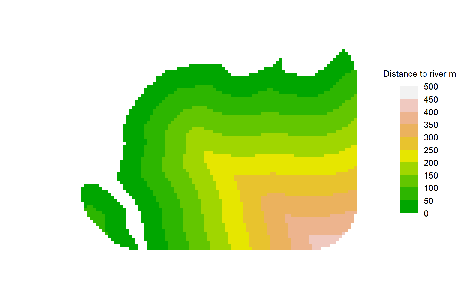
11.3.5 Pre-computed resource selection functions
A resource selection function (RSF) was defined by Boyce et al. (2002) as “any model that yields values proportional to the probability of use of a resource unit”. An RSF combines habitat information from multiple sources in a single variable. Typically the function is estimated from telemetry data on marked individuals, and primarily describes individual-level behaviour (3rd-order habitat selection of Johnson, 1980).
However, the individual-level RSF is also a plausible hypothesis for 2nd-order habitat selection i.e. for modelling the relationship between habitat and population density. Then we interpret the RSF as a single variable that is believed to be proportional to the expected population density in each cell of a habitat mask. For example, Proffitt et al. (2015) used an RSF developed independently from telemetry data on utilisation in relation to terrain and land cover to model spatial variation in the density of mountain lions Puma concolor in Montana.
Suppose, for example, in folder datadir we have a polygon shapefile (RSF.shp, RSF.dbf etc.) with the attribute “rsf” defined for each polygon. Given mask and capthist objects “habmask” and “myCH”, this code fits a SECR model that calibrates the RSF in terms of population density:
- “rsf” must be known for every pixel in the habitat mask
- Usually it make sense to fit the density model through the origin (rsf = 0 implies D = 0). This is not true of habitat suitability indices in general.
This is a quite different approach to fitting multiple habitat covariates within secr, and one that should be considered. There are usually too few individuals in a SECR study to usefully fit models with multiple covariates of density, even given a large dataset such as our possum example. However, 3rd-order and 2nd-order habitat selection are conceptually distinct, and their relationship is an interesting research topic (e.g., Linden et al., 2018).
11.3.6 Regression splines
Regression splines are a flexible alternative to polynomials for spatial trend analysis. Regression splines are familiar as the smooth terms in ‘generalized additive models’ (gams) implemented (differently) in the base R package gam and in R package mgcv (Wood, 2006).
Some of the possible smooth terms from mgcv can be used in model formulae for secr.fit – see the help page for ‘smooths’ in secr. Smooths are specified with terms that look like calls to the functions s and te. Smoothness is determined by the number of knots which is set by the user via the argument ‘k’. The number of knots cannot be determined automatically by the penalty algorithms of mgcv.
Here we fit a regression spline with the same number of parameters as a quadratic polynomial, a linear effect of the ‘distance to river’ covariate on log(D), and a nonlinear smooth.
Now add these to the AIC table and plot the ‘AIC-best’ model:
        npar   logLik  dAIC  AICwt
RS3        5 -1552.00 0.000 0.2667
Dxy2       8 -1549.32 0.628 0.1948
RS2        4 -1553.36 0.705 0.1875
Dxy        5 -1552.86 1.714 0.1132
RS1        8 -1549.93 1.847 0.1059
Dforest    4 -1554.15 2.281 0.0853
null       3 -1555.75 3.488 0.0466
newdat <- data.frame(DTR = seq(0,400,5))
tmp <- predict(RSfits$RS3, newdata = newdat)
par(mar=c(5,8,2,4), pty = "s")
plot(seq(0,400,5), sapply(tmp, "[", "D","estimate"),
ylim = c(0,20), xlab = "Distance from river (m)",
ylab = "Density / ha", type = "l")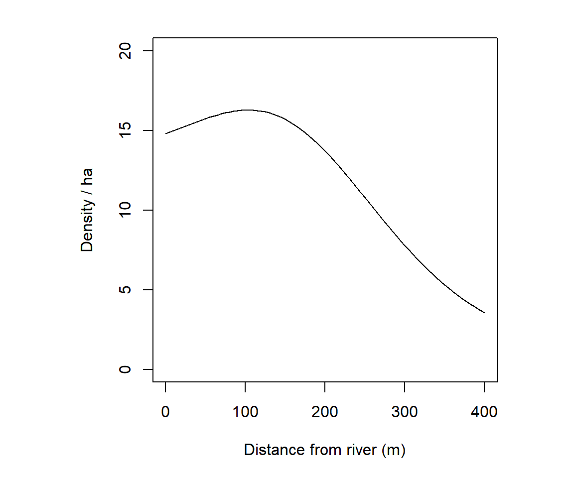
Confidence intervals are computed in predictDsurface by back-transforming \pm 2SE from the link (log) scale:
code for lower and upper confidence surfaces
par(mar = c(1,1,1,1), mfrow = c(1,2), xpd = FALSE)
surfaceDDTR3 <- predictDsurface(RSfits$RS3, cl.D = TRUE)
plot(surfaceDDTR3, covariate= "lcl", breaks = seq(0,22,2),
    legend = FALSE)
mtext(side = 3,line = -1.5, cex = 0.8,
      "Lower 95% confidence limit of D (possums / ha)")
plot(surfaceDDTR3, plottype = "contour", breaks = seq(0,22,2),
    add = TRUE)
lines(leftbank)
plot(surfaceDDTR3, covariate= "ucl", breaks = seq(0,22,2),
    legend = FALSE)
mtext(side = 3, line = -1.5, cex = 0.8,
    "Upper 95% confidence limit of D (possums / ha)")
plot(surfaceDDTR3, covariate = "ucl", plottype = "contour",
    breaks = seq(0,22,2), add = TRUE)
lines(leftbank)
mtext(side=3, line=-1, outer=TRUE, "s(DTR, k = 3) model", cex = 0.9)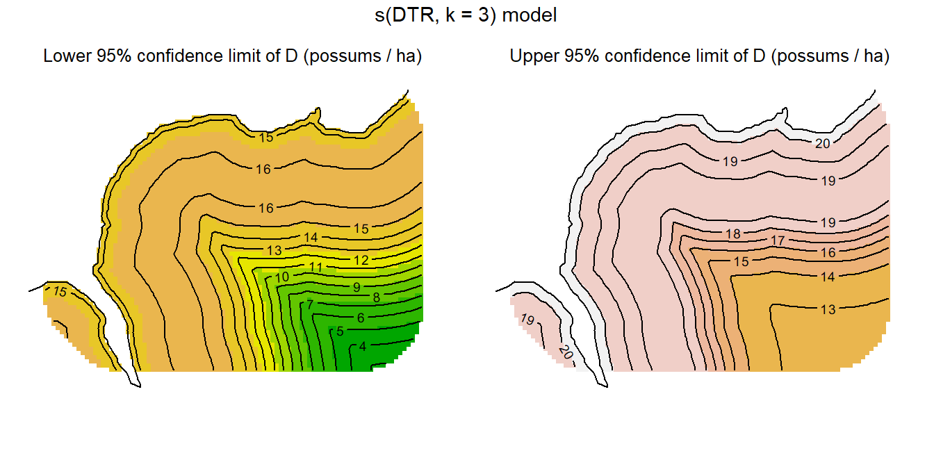
Multiple predictors may be included in one ‘s’ smooth term, implying interaction. This assumes isotropy – equality of scales on the different predictors – which is appropriate for geographic coordinates such as x and y in this example. In other cases, predictors may be measured on different scales (e.g., structural complexity of vegetation and elevation) and isotropy cannot be assumed. In these cases a tensor-product smooth (te) is appropriate because it is scale-invariant. For te, ‘k’ represents the order of the smooth on each axis, and we must fix the number of knots with ‘fx = TRUE’ to override automatic selection.
For more on the use of regression splines see the documentation for mgcv, the secr help page `?smooths’, Wood (2006), and Borchers & Kidney (2014).
11.3.7 Scale of effect
Modelling density as a function of covariate(s) at a point (the centroid of a mask cell) lacks biological realism. Individuals exploit resources across their home range, and density may be affected by regional dynamics over a much wider area (e.g., Jackson & Fahrig, 2014).
The scale at which environmental predictors influence density is usually unknown, and almost certainly does not correspond to either a point or the arbitrary size of a mask cell. Some progress has been made in estimating the scale from data (e.g., Chandler & Hepinstall-Cymerman, 2016), but methods have not yet been integrated into SECR.
The best we can do at present is to construct spatial layers in GIS software that represent various levels of smoothing or spatial aggregation, corresponding to different scales of effect. Each layer may then be imported as a mask covariate that is evaluated at the cell centroids to represent the surrounding area.
This example uses the focal function in the terra package (Hijmans, 2023) to compute both the proportion of forest cells in a square window and a Gaussian-smoothed proportion.
code for smoothed covariates
# binary SpatRaster 0 = nonbeech, 1 = beech
covariates(ovmask)$forest_num <- ifelse (covariates(ovmask)$forest == 'beech', 1,0)
tmp <- terra::rast(ovmask, covariate = 'forest_num')

# square smoothing window: 5 cells
tmpw5 <- terra::focal(tmp, w = 5, "mean", na.policy = "omit", na.rm = TRUE)
names(tmpw5) <- 'w5'

# Gaussian window, sigma 50 m
# window radius is 3 sigma
g50 <- terra::focalMat(tmp, d = 50, type = "Gauss")
tmpg50 <- terra::focal(tmp, w = g50, "sum", na.policy = "omit", na.rm = TRUE)
names(tmpg50) <- 'g50'

# add to mask
ovmask <- addCovariates(ovmask, tmpw5)
ovmask <- addCovariates(ovmask, tmpg50)

# plot
par(mar = c(1,1,1,1), mfrow = c(1,2), xpd = FALSE)

plot(ovmask, cov = 'w5', dots = FALSE, legend = FALSE)
plot(ovtrap, add = TRUE)
text (2674600, 5982892, 'a.', cex = 1.2)

plot(ovmask, cov = 'g50', dots = FALSE, legend = FALSE)
plot(ovtrap, add = TRUE)
text (2674600, 5982892, 'b.', cex = 1.2)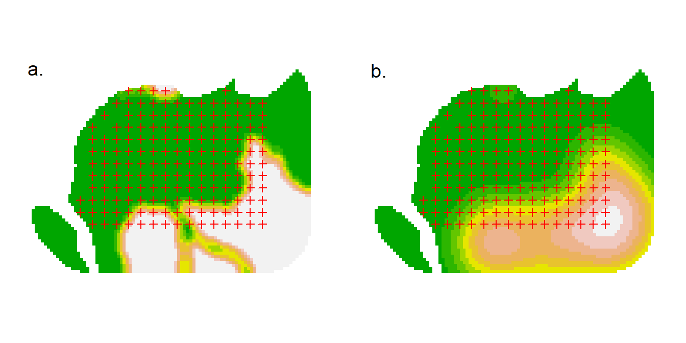
11.4 Prediction and plotting
Fitting a model provides estimates of its coefficients or ‘beta parameters’; use the coef method to extract these from an secr object. The coefficients are usually of little use in themselves, but we can use them to make predictions. In order to plot a fitted model we first predict the height of the density surface at each point on a mask. As we have seen, this is done with predictDsurface, which has arguments (object, mask = NULL, se.D = FALSE, cl.D = FALSE, alpha = 0.05). By default, prediction is at the mask points used when fitting the model (i.e. object$mask); specify the mask argument to extrapolate the model to a different area.
The output from predictDsurface is a specialised mask object called a Dsurface (class “c(‘Dsurface’, ‘mask’, ‘data.frame’)”). The covariate dataframe of a Dsurface has columns for the predicted density of each group (D.0 if there is only one). Usually when you print a mask you see only the x- and y-coordinates. The print method for Dsurface objects displays both the coordinates and the density values as one dataframe, as also do the head and tail methods.
Use the arguments ‘se.D’ and ‘cl.D’ to request computation of the estimated standard error and/or upper and lower confidence limits for each mask point3. If requested, values are saved as additional covariates of the output Dsurface (SE.0, lcl.0, and ucl.0 if there is only one group).
The plot method for a Dsurface object has arguments (x, covariate = "D", group = NULL, plottype = "shaded", scale = 1, ...). covariate may either be a prefix (one of “D”, “SE”, “lcl”, “ucl”) or any full covariate name. ‘plottype’ may be one of “shaded”, “dots”, “persp”, or “contour”. A coloured legend is displayed centre-right (see ?plot.mask and ?strip.legend for options).
For details on how to specify colours, levels etc. read the help pages for plot.mask, contour and persp (these functions may be controlled by extra arguments to plot.Dsurface, using the ‘dots’ convention).
A plot may be enhanced by the addition of contours. This is a challenge, because the contour function in R requires a rectangular matrix of values, and our mask is not rectangular. We could make it so with the secr function rectangularMask, which makes a rectangular Dsurface with missing (NA) values of density at all the external points. plot.Dsurface recognises an irregular mask and attempts to fix this with an internal call to rectangularMask.
11.5 Scaling
So far we have ignored the scaling of covariates, including geographic coordinates.
secr.fit scales the x- and y-coordinates of mask points to mean = 0, SD = 1 before using the coordinates in a model. Remember this when you come to use the coefficients of a density model. Functions such as predictDsurface take care of scaling automatically. predict.secr uses the scaled values (‘newdata’ x = 0, y = 0), which provides the predicted density at the mask centroid. The mean and SD used in scaling are those saved as the `meanSD’ attribute of a mask (dataframe with columns ‘x’ and ‘y’ and rows ‘mean’ and ‘SD’).
Scaling of covariates other than x and y is up to the user. It is not usually needed.
The numerical algorithms for maximizing the likelihood work best when the absolute expected values are roughly similar for all parameters on their respective ‘link’ scales (i.e. all beta parameters) rather than varying by orders of magnitude. The default link function for D and sigma (log) places the values of these parameters on a scale that is not wildly different to the variation in g0 or lambda0, so this is seldom an issue. In extreme cases you may want to make allowance by setting the typsize argument of nlm or the parscale control argument of optim (via the … argument of secr.fit).
Scaling is not performed routinely by secr.fit for distance calculations. Sometimes, large numeric values in coordinates can cause loss of precision in distance calculations (there are a lot of them at each likelihood evaluation). The problem is serious in datasets that combine large coordinates with small detector spacing, such as the Lake Station skink dataset. Set details = list(centred = TRUE) to force scaling; this may become the default setting in a future version of secr.
11.6 This is not a density surface
The surfaces we have fitted involve inhomogeneous Poisson models for the distribution of animal home range centres. The models have parameters that determine the relationship of expected density to location or to habitat covariates.
Another type of plot is sometimes presented and described as a ‘density surface’ – the summed posterior distribution of estimated range centres from a Bayesian fit of a homogeneous Poisson model. A directly analogous plot may be obtained from the secr function fxTotal (see also Borchers & Efford (2008) Section 4.3). The contours associated with the home range centre of each detected individual essentially represent 2-D confidence intervals for its home range centre, given the fitted observation model. Summing these gives a summed probability density surface for the centres of the observed individuals (‘D.fx’), and to this we can add an equivalent scaled probability density surface for the individuals that escaped detection (‘D.nc’). Both components are reported by fx.total, along with their sum (‘D.sum’) which we plot here for the flat possum model:
fxsurface <- fxTotal(fits$null)par(mar = c(1,6,2,8))
plot(fxsurface, covariate = "D.sum", breaks = seq(0,30,2),
poly = FALSE)
plot(ovtrap, add = TRUE)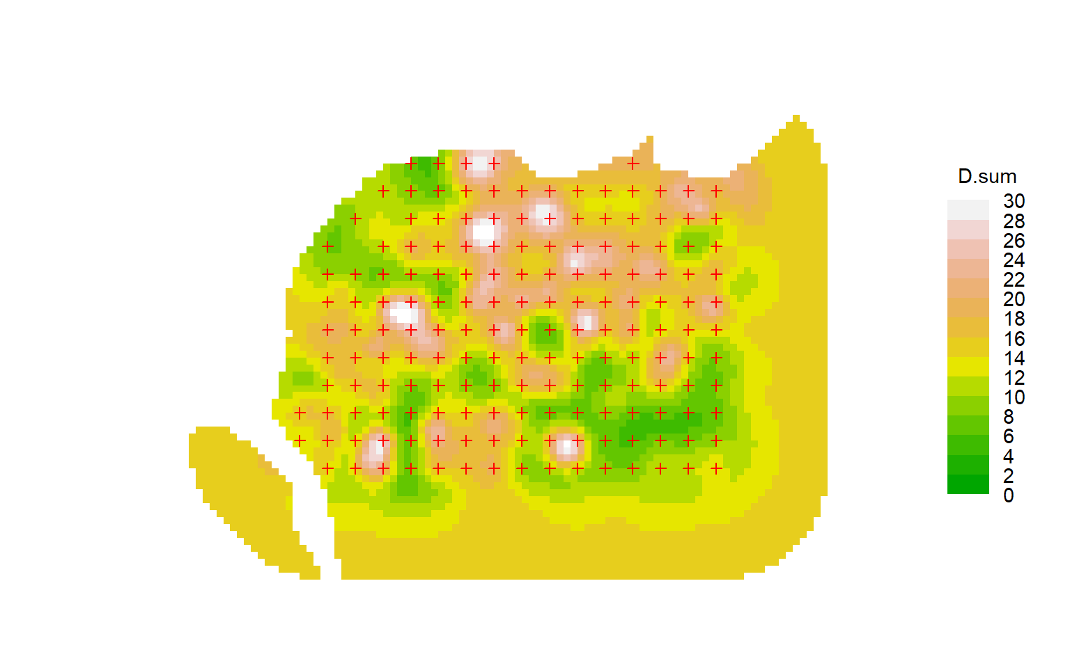
The plot concerns only one realisation from the underlying Poisson model. It visually invites us to interpret patterns in that realisation that we have not modelled. There are serious problems with the interpretation of such plots as ‘density surfaces’:
attention is focussed on the individuals that were detected; others that were present but not detected are represented by a smoothly varying base level that dominates in the outer region of the plot (contrast this figure with the previous quadratic and DTR3 models).
the surface depends on sampling intensity, and as more data are added it will change shape systematically. Ultimately, the surface near the centre of a detector array becomes a set of emergent peaks rising from an underwater plain of zero density, below the plateau of average density outside the array.
the ‘summed confidence interval’ plot is easily confused with the 2-D surface obtained by summing utilisation distributions across animals
confidence intervals are not available for the height of the probability density surface.
The plots are also prone to artefacts. In some examples we see concentric clustering of estimated centres around the trapping grids, apparently ‘repelled’ from the traps themselves (e.g., plot below for a null model of the Waitarere ‘possumCH’ dataset in secr). This phenomenon appears to relate to lack of model fit (unpubl. results).
fxsurfaceW <- fxTotal(possum.model.0)par(mar = c(1,5,1,8))
plot(fxsurfaceW, covariate = "D.sum", breaks = seq(0,5,0.5),
poly = FALSE)
plot(traps(possumCH), add = TRUE)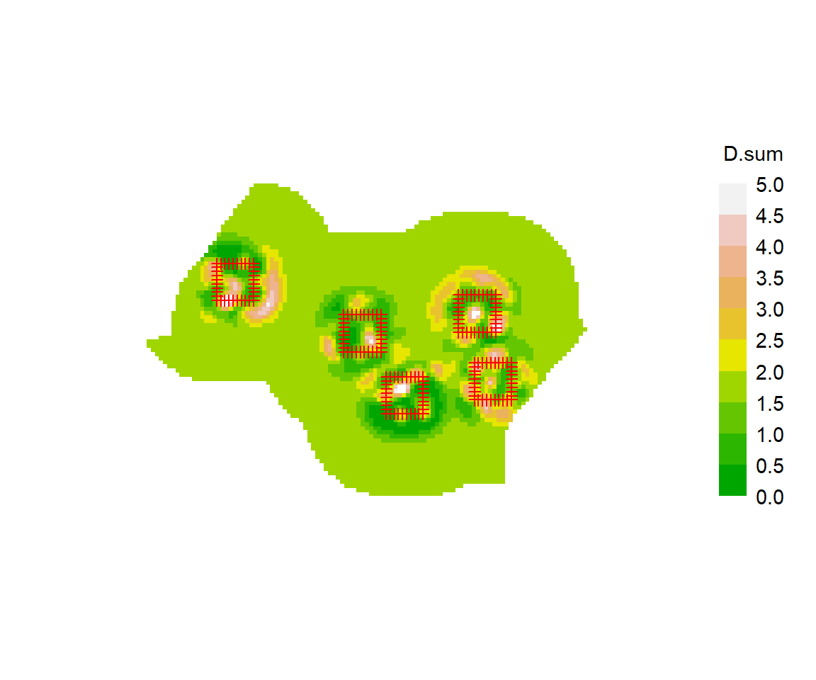
See Durbach et al. (2024) for further critique.
11.7 Relative density
Theory for relative density models was given earlier (see also (Efford, 2025)). A spatial model for relative density is fitted in secr by setting CL = TRUE and providing a model for D in the call to secr.fit (secr \ge 5.2.0). For example
fitrd1 <- secr.fit(capthist = OVpossumCH[[1]], mask = ovmask,
    trace = FALSE, model = D ~ x + y + x2 + y2 + xy, CL = TRUE)
options(digits = 4)
coef(fitrd1)[,1:2]
beta SE.beta
D.x -0.19871 0.11851
D.y 0.30998 0.13469
D.x2 -0.22472 0.13345
D.y2 -0.09673 0.12818
D.xy 0.29672 0.13208
g0 -2.22032 0.09422
sigma 3.31767 0.03544# compare coefficients from full fit:
coef(fits$Dxy2)[1:2] beta SE.beta
D 2.72538 0.12781
D.x -0.19871 0.11851
D.y 0.30999 0.13468
D.x2 -0.22471 0.13344
D.y2 -0.09674 0.12817
D.xy 0.29672 0.13208
g0 -2.22032 0.09422
sigma 3.31767 0.03544The relative density model is fitted by maximizing the likelihood conditional on n and has one fewer coefficients than the absolute density model. Estimates of other coefficients are the same within numerical error (log link) or are scaled by the intercept (identity link).
The density intercept and other coefficients may be retrieved with the function derivedDcoef:
derivedDcoef(fitrd1) # delta-method variance suppressed as unreliable beta SE.beta lcl ucl
D 2.7253890 NA NA NA
D.x -0.1987149 0.1185098 -0.4309898 0.0335599
D.y 0.3099849 0.1346873 0.0460026 0.5739672
D.x2 -0.2247201 0.1334477 -0.4862729 0.0368326
D.y2 -0.0967319 0.1281839 -0.3479677 0.1545040
D.xy 0.2967233 0.1320827 0.0378459 0.5556006
g0 -2.2203193 0.0942197 -2.4049865 -2.0356520
sigma 3.3176747 0.0354359 3.2482216 3.3871277To plot the full density surface it is first necessary to infer the missing intercept. This is done automatically by the function derivedDsurface:
par(mar = c(1,6,2,8))
derivedD <- derivedDsurface(fitrd1)
plot(derivedD, plottype = "shaded", poly = FALSE, breaks =
      seq(0,22,2), title = "Density / ha", text.cex = 1)
plot(surfaceDxy2, plottype = "contour", poly = FALSE, breaks =
    seq(0,22,2), add = TRUE)
lines(leftbank)
The density in Fig. 11.9 nearly matches the absolute density in Fig. 11.2. This will not be the case if the relative density model is fitted to data from animals tagged elsewhere or on a subset of the area. Tagging then imposes differential spatial weighting that must be made explicit in the model to recover the correct pattern of density in relation to covariates. One scenario involves acoustic telemetry or other automated detection for which the only animals at risk of detection are those previously marked (cf resighting data, in which unmarked animals are detected and counted, but not identified).
We can also express the model as before \mathbf y = \mathbf X \pmb {\beta}, where \mathbf X is the design matrix, \pmb{\beta} is a vector of coefficients, and \mathbf y is the resulting vector of densities on the link scale. Rows of \mathbf X and elements of \mathbf y correspond to points on the habitat mask, possibly replicated in the case of group and session effects.↩︎
It may also be specified in a user-written function supplied to
secr.fit(see Appendix I), but you are unlikely to need this.
↩︎Option available only for models specified in generalized linear model form with the ‘model’ argument of secr.fit, not for user-defined functions.↩︎