8 Study design
Study design for SECR brings together many disparate considerations, some external to SECR itself (goals, cost, logistics). In this chapter we hope to build an understanding of the working properties of SECR and integrate the external considerations into a strategy for effective study design.
Defining the area of interest is a necessary first step towards rational study design. By ‘area of interest’ we mean the geographic region for which an estimate of population density or population size is required. When the goal is to characterise the density of a species in a particular habitat it is tempting to think that “any patch will do”, but defining the area, and hence the scope of inference, is an important discipline. Even when the primary goal is to infer the relationship between density and habitat covariates, rather than to estimate average density or population size, defining a region ties the model to particular patterns of variation in the covariates. Goals, cost, logistics, and tradeoffs among these factors, will determine the area of interest. These are study-specific, so we cannot say much more here.
The key design variables are the choice of methods for detection and individual identification, the number and placement of detectors, and the duration of sampling. The available detection and identification methods vary from taxon to taxon, and we do not consider them in detail. Cost is an ever-present constraint on the remaining variables, but we leave it to the end.
Tools for study design are provided in the R package secrdesign and its online interface secrdesignapp. Simulation of candidate designs is a central method, but for clarity we defer instruction on that until Chapter 17.
8.1 Studies focussing on design
General issues of study design for SECR were considered by Sollmann et al. (2012), Tobler & Powell (2013), Sun et al. (2014), Clark (2019), and Efford & Boulanger (2019). Algorithmic optimisation of detector locations was described by Dupont et al. (2021) and Durbach et al. (2021). Design issues appeared incidentally in Efford et al. (2005), Efford & Fewster (2013), Noss et al. (2012), and Palmero et al. (2023), among other papers.
8.2 Data requirements for SECR
We list here some minimum data requirements that might be labelled “assumptions” but are more fundamental. They should be addressed by appropriate study design.
Requirement 1. Sampling representative of the area of interest
This requirement is important and easy to overlook. The problem takes care of itself when detectors are placed evenly throughout the area of interest, exposing all individuals to a similar probability of detection. This is usually too costly when the area of interest is large. Sub-sampling is then called for, and we consider the options later.
Deliberate, statistically non-representative, placement of detectors may be justified in certain studies, specifically when the goal is to infer the relationship between density and habitat variables. It is then optimal to sample along the environmental gradients of interest. We do not address study design for this case.
More on modelling as an alternative to representative sampling
Our emphasis on representative and spatially balanced sampling may seem over-the-top. SECR is model-based and the variance estimates make no assumptions regarding the sampling design. Sampling deliberately across environmental gradients may well provide the best information on particular covariate effects, and a fitted model with these covariates may be extrapolated across the area of interest to estimate average density. Nevertheless, we advocate representative sampling because it protects against vulnerabilities of a purely model-based approach:
- density may be non-uniform for reasons not related to any observable covariate (e.g., historical disease outbreaks)
- spatial variation in detection parameters (\lambda_0, \sigma) is often omitted from models
- covariates are not causal, and different correlations may apply in unsampled parts of the region
- extrapolation to values of the covariate(s) that are rare or absent in the data is risky, especially with the log-linear models commonly used.
Requirement 2. Many individuals detected more than once
This requirement is common to all capture–recapture methods. Estimation of detection parameters conditions on the first detection, and detections after the first are needed to estimate a non-zero detection rate. The question ‘How many is enough?’ is addressed later.
Requirement 3. Spread adequate to estimate spatial scale of detection
By ‘spread’ we mean the spatial extent of the detections of an individual. The spread of detections must be adequate in two respects:
Requirement 3a. Some individuals are detected at more than one detector, and
Requirement 3b. Detections of an individual should be localised to part of the detector array.
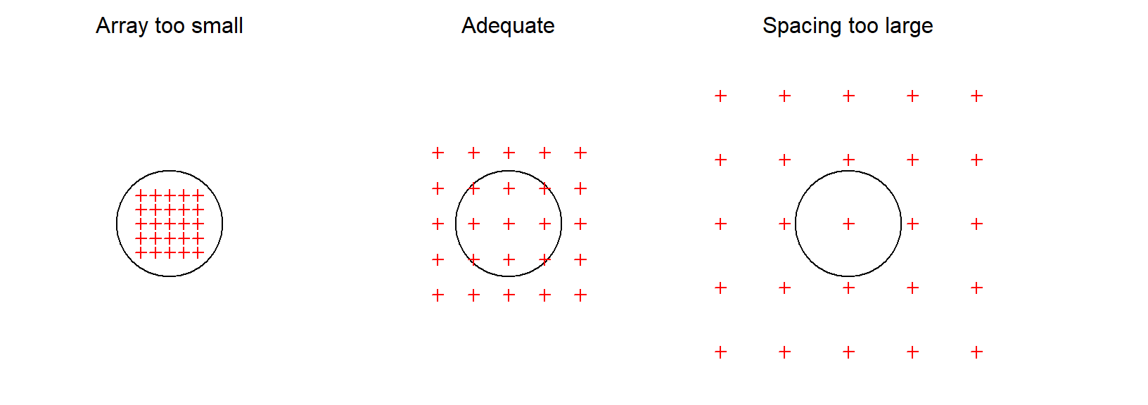
Adequate spread is achieved by matching the size and spacing of a detector array to the scale of movement, as shown schematically in Fig. 8.1.
Some qualification is needed here. We require only that some individuals, a representative sample, are detected at more than one detector, and that the detector array is large enough to differentiate points in the middle and edge of some home ranges. Failure to meet the ‘spread’ requirement may be addressed, at least in principle, by combining SECR and telemetry, but improved study design is a better solution.
A poorly designed detector array may give data that cannot be analysed by SECR, or provide highly biased estimates of low precision. Such designs were described by Efford & Boulanger (2019) as ‘pathological’. We seek a non-pathological and representative design that gives the most precise estimates possible for a given cost.
8.3 Precision and power
Precise estimates have narrow confidence intervals and high power to detect change. Precision and bias jointly determine the accuracy of estimates, measured by the root-mean-square error (the difference between estimates and the true value). Bias is typically a minor component, and for now we assume it is negligible.
Precision is conveniently measured by its inverse, the relative standard error (RSE) where \mathrm{RSE}(\hat \theta) = \widehat{\mathrm{SE}}(\hat \theta) / {\hat \theta} for estimate \hat \theta of parameter \theta. In statistics, the standard error is the square root of the sampling variance, estimated for MLE as described in Section 3.6. Wildlife papers often use ‘CV’ for the RSE of estimates, but this confuses relative standard error and relative standard deviation.
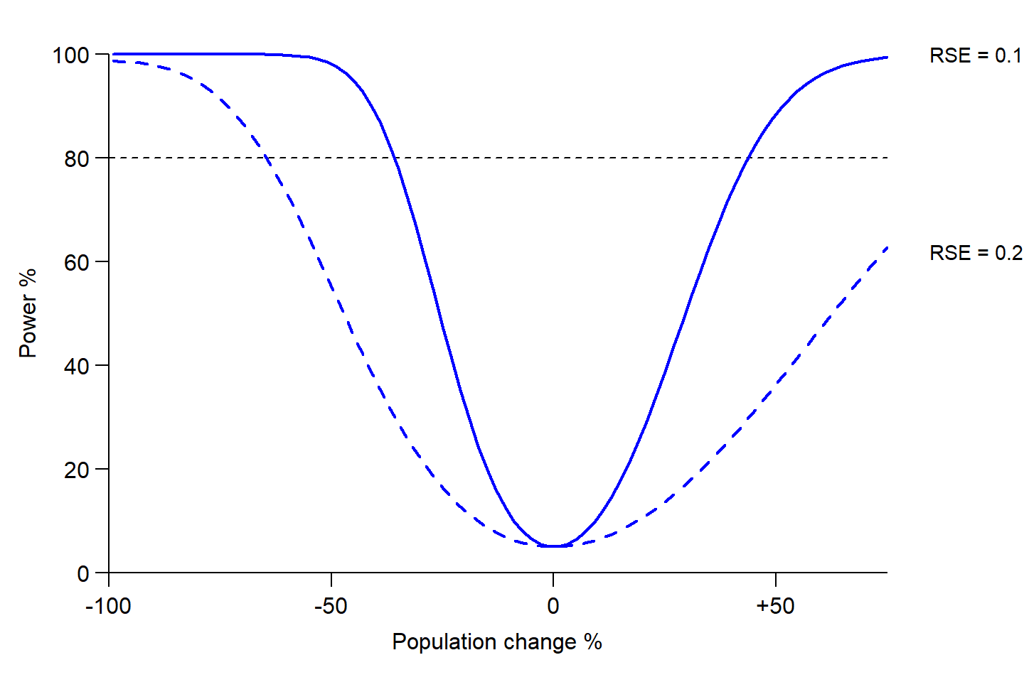
The question ‘What precision do I need?’ requires clarity on the purpose of the study. If the purpose is to compare density estimates from different times or places with the same effort then the power to detect change of a given magnitude is a direct function of the initial \mathrm{RSE}(\hat D) (Fig. 8.2). Although RSE = 0.2 is often touted as adequate “for management purposes”, estimates with RSE = 0.2 have low (\le 50%) power to detect a change in density of even \pm 50% at the usual \alpha = 0.05 (Fig. 8.2). If reliable estimates are vital for population management, as claimed routinely in methodological papers, then surely greater precision is required. RSE = 0.1 is a better general target.
We lack a clear guide to required RSE in other studies, for which the effect size may be ill-defined. We have observed that fitted models with \mathrm{RSE}(\hat D) \gg 0.2 behave erratically with respect to AIC model selection, presumably because of sampling variance in the AIC values themselves.
8.4 Pilot parameter values
To evaluate a potential study design we must know something about the target population. Here we describe the population and the behaviour of individuals by a simple SECR model and its parameters: uniform density D and the parameters \lambda_0 and \sigma of a hazard half-normal detection function. Predictions regarding the suitability and performance of any design then depend on the values of D, \lambda_0 and \sigma. This seems like a catch-22 – impossible until we have estimates – but for design purposes we can call on approximate values from multiple sources
- published estimates from studies of similar species,
- a low-precision pilot study, or
- indirect inference.
Reviews of SECR studies are a useful source of pilot estimates (e.g., Palmero et al., 2023). The hardest parameter to pin down is \lambda_0, as this is very study-specific. The good news is that it has only a secondary effect on the relative merits of different array designs.
hazard \lambda_0 vs probability g_0
We emphasise hazard detection functions (intercept \lambda_0) over probability detection functions (intercept g_0) because the formulae for expected counts are straightforward (Appendix K). However, pilot values of the probability parameters are more commonly available. Note that the fitted \sigma also differs. For design purposes, the parameters of the probability detection function (g_0, \sigma) may be substituted for the corresponding parameters of the hazard detection functions (\lambda_0, \sigma). If desired, the internal function dfcast of secrdesign provides a more precise match e.g., secrdesign:::dfcast(detectfn = 'HN', detectpar=list(g0 = 0.2, sigma = 25))
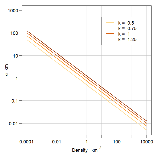
Indirect inference is a murky option, but better than nothing, and there are some constraints. The quantity k = \sigma \sqrt D (loosely described by Efford et al. (2016) as an index of home range overlap) usually falls in the range 0.3–1.3 for solitary species (M. Efford unpubl.). secr expresses D in animals / ha and \sigma in metres, so a factor of 100 is needed, and \sigma = \frac{100}{\sqrt{2D}} is a good start (k \approx 0.707).
We can use the close analogy between the detection function and a home-range utilisation distribution to extract a pilot value of \sigma from home range data. Most directly, a circular bivariate normal (BVN) model can be fitted to telemetry data; we then use the dispersion parameter directly as a pilot value of \sigma for hazard half-normal detection. If the home range data have been summarised as the area a within a notional 95% activity contour then the spatial scale parameter of the hazard half-normal is close to \sigma = \sqrt \frac{a}{6 \pi} (Jennrich & Turner, 1969 Eq. 13)1.
Scalability
Simulation to compare study designs commonly rests on the assumption that the underlying detection process is constant. If parameters vary between layouts in a way not captured by the model (see salamander example) then extrapolation to novel layouts is unreliable. There is an analogous problem when locations are serially correlated: estimates of detection parameters (especially \sigma) are then specific to the duration of the pilot study and cannot safely be extrapolated to other durations.
8.5 Expected sample size
Given some pilot parameter values, we might proceed directly to simulating data from different designs and computing the resulting SECR estimates. This is effective, but slow. A useful preliminary step is to check the expected sample size of potential designs.
The sample size for SECR is more than a single number. We suggest calculating the expected values of these count statistics:
- n the number of distinct individuals detected at least once,
- r the total number of re-detections (any detection after an individual is first detected), and
- m the total number of movements (re-detections at a detector different to the preceding one).
The counts depend on the detector configuration, the extent of habitat (buffer width), and the type of detector (trap, proximity detector etc.) in addition to the parameter values. Formulae are given in Appendix K. Calculation is fast and the counts give insight on whether the data generated by a design are likely to be adequate. E(r) is a direct measure of Requirement 2 above. E(m) addresses Requirement 3a (‘Spacing too large’ in Fig. 8.1).
Spatial recaptures
The term ‘spatial recaptures’ corresponds loosely with our m. Spatial recaptures are a sine qua non of SECR, but their role in determining precision can be overstated. They are a consequence of Requirements 2 and 3, not an independent effect. Furthermore:
i. Movements are ill-defined when detections are aggregated by time, as then we cannot distinguish the capture histories ABABA and AAABB at detectors A and B (both are (3A, 2B), but one implies 4 movements and the other one).
ii. Spatial and non-spatial recaptures have barely distinguishable effects when detectors are very close; a profusion of close spatial recaptures is not very useful (e.g., Durbach et al., 2021).
8.6 A useful approximation
Efford & Boulanger (2019) found that E(n) and E(r) alone were often sufficient to predict the precision of SECR density estimates. The relationship is
\mathrm{RSE}(\hat D) \approx 1 / \sqrt{\mathrm{min} \{ \mathrm{E}(n), \mathrm{E}(r)\} }. This formula supports intuition regarding the effect of particular designs on precision, especially the ‘n–r tradeoff’ described later. Computation is much faster than estimating \hat D. The approximation is used in the interactive Shiny application secrdesignapp and for algorithmic optimisation (Durbach et al., 2021). Limitations and refinements are discussed in the papers cited.
8.7 Array size versus home range
We lack a count statistic matching the second part of Requirement 3 (‘Array too small’ in Fig. 8.1). We therefore define an ad hoc measure of sampling scale that we call the ‘extent ratio’: this is the diameter of the array (the distance between the most extreme detectors) divided by the nominal diameter of a 95% home range. The 95% home-range radius is r_{0.95} \approx 2.45 \sigma for a BVN utilisation distribution (from the previous formula).
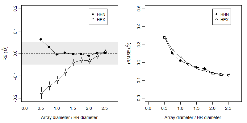
Simulations described on GitHub show that SECR performs poorly when the extent ratio is less than 1: the relative bias and root-mean-square error of \hat D increase abruptly (Fig. 8.4). We earlier touted the robustness of \hat D to misspecification of the detection function, but this desirable property evaporates when the array is small, as shown by estimates from a hazard exponential function applied to hazard half-normal data in Fig. 8.4.
Efford (2011) simulated area-search data for a range of area sizes. Plotting those results with the extent ratio as the x-axis shows a similar pattern to Fig. 8.4 (see GitHub).
The extent ratio does not provide a precise criterion because it combines two somewhat arbitrary measures (array diameter, 95% home range diameter). What the simulations reveal about array size can be summed up in a simple rule: the grid or searched area should be at least the size of the home range, and larger arrays provide greater robustness and accuracy.
8.8 The n-r tradeoff
The performance of the SECR density estimator depends on both the number of individuals n and the number of re-detections r. However, we cannot maximise their expected values simultaneously. E(n) is greatest when detectors are far apart and each detector samples a different set of individuals (AC). For binary proximity detectors E(r) is greatest when detectors are clumped together and declines monotonically with spacing; for multi-catch traps, E(r) increases and then declines (Fig. 8.5).
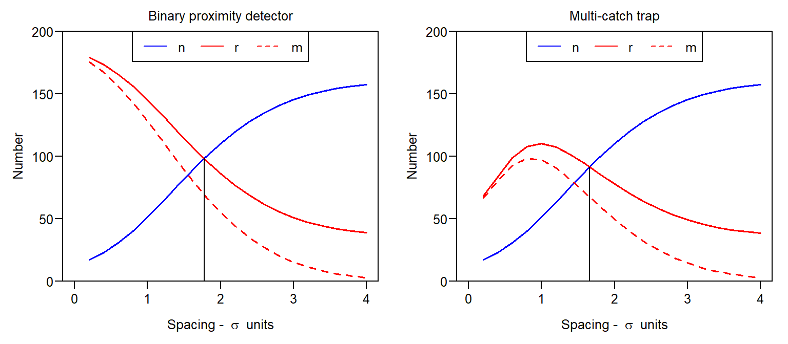
To maximise the sample size we seek a satisfactory compromise, an intermediate spacing of detectors that yields both high E(n) and high E(r). There is so far no evidence for weighting one more than the other; later simulations suggest aiming for E(n) \approx E(r), as indicated by the vertical lines in Fig. 8.5. The number of movement recaptures m follows the pattern of total recaptures r and need not be considered separately.
8.9 Spacing and precision
We expect precision to improve with sample size. From the last section we understand that sample size depends somewhat subtly on detector spacing: wider spacing increases n because a larger area is sampled, but it ultimately reduces r. We next use simulation to demonstrate the effect on the precision. We measure precision by the relative standard error of density estimates \mathrm{RSE} (\hat D). In the following examples we assume a Poisson distribution for n rather than the binomial distribution that results when N(A) is fixed.
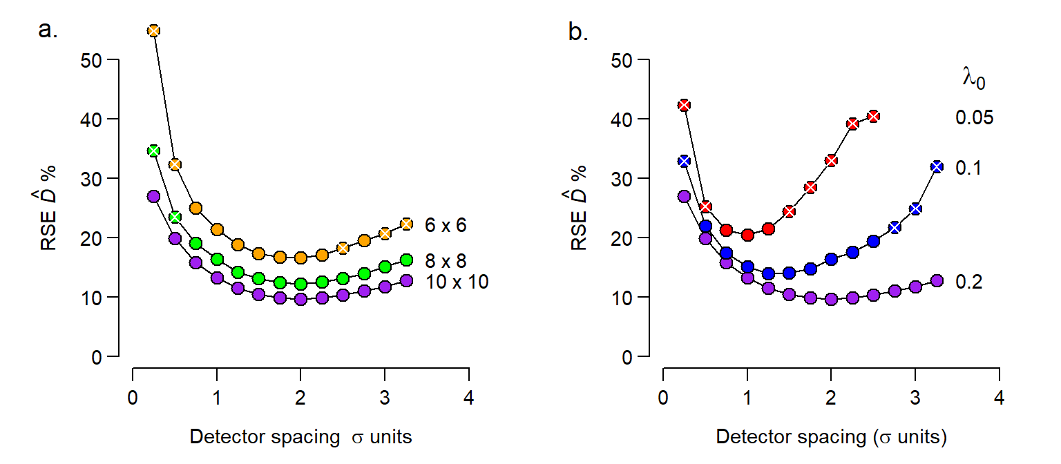
The simulations in Fig. 8.6 are representative: there is an optimal spacing (often around 2\sigma for a hazard half-normal detection function) and a broad range of spacings yielding similar precision. The optimum is close, but not identical, to the spacing that gives E(n) = E(r) in Fig. 8.5. The variability of the simulations increases away from the optimum spacing: if we are in the right ballpark then very few replicates are needed to capture it.
Although 2\sigma is often mentioned as an optimum, the optimal spacing is smaller when sampling intensity is low. This happens when there are few sampling occasions or \lambda_0 is small, as illustrated in Fig. 8.6.
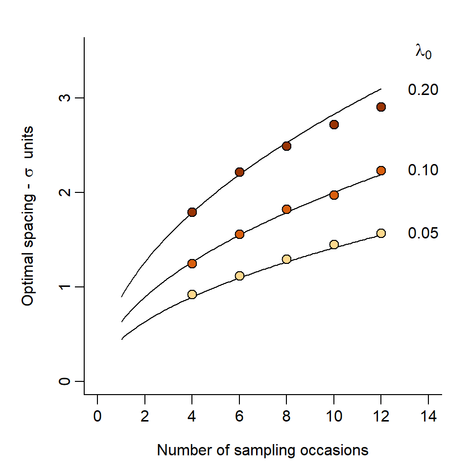
The curves in Fig. 8.7 are given by R_{opt} = 2 \sqrt{\lambda_0 S} where R_{opt} is the optimal spacing in \sigma units and S is the number of occasions. The reason for this apparently tight relationship has yet to be determined, and it is unreliable for intensive sampling (large S\lambda_0), as indicated by the simulations for \lambda_0 = 0.2 and S \ge 10.
8.10 Detectors required for uniform array
Increasing imprecision of \hat D and failure of estimation in many cases (indicated by white crosses in Fig. 8.6) place a limit on the size of region A that can be sampled with a uniform grid of K detectors. At the optimum spacing (i.e. about 2\sigma\sqrt{\lambda_0 S}) we require K > A / (4\sigma^2\lambda_0 S).
A region of interest with area A \gg 4K\sigma^2 \lambda_0 S cannot be covered adequately with a uniform grid of K detectors. Thus for binary proximity detectors and hazard half-normal detection with \lambda_0 = 0.1,
- when \sigma = 50 m, sampling with 100 detectors for S = 5 occasions covers 50 ha at 71-m spacing
- when \sigma = 1 km (implying larger home range and lower density), then sampling with 100 detectors for S = 5 occasions covers 200 km2 at 1.4-km spacing.
The spacing may be stretched somewhat from the optimum if we are willing to accept suboptimal precision, but increasing spacing by more than 50% also runs the risk of bias (Fig. 8.6).
The ratio R_K = 4\sigma^2K/A is a useful guide for planning, where K is the number of detectors that can be deployed. R_K \ge 1.0 allows for a uniform grid, whereas for R_K \ll 1.0 there are too few detectors for an efficient uniform grid. Here we assume \sqrt{\lambda_0 S}\approx 1.0.
8.11 Number of detectors in fixed region
We have referred to 2\sigma\sqrt{\lambda_0 S} as an ‘optimum’ spacing for the scenario that the number of detectors is fixed. Increasing the number of detectors in an area of interest can be expected to increase sample sizes, particularly \mathrm E(r), and hence to improve on precision beyond the ‘optimum’. For a non-arbitrary area R_K > 1.0 is entirely appropriate, and cost becomes the decider. The benefit from increasing the density of detectors may be small; for example, trebling the number of detectors in a 10-ha area from K_0 = A / (4\sigma^2\lambda_0 S) = 62.5 resulted in only a 27% reduction in \mathrm{RSE}(\hat D) for the base parameter values of Fig. 8.5.
8.12 Clustered designs
We have assumed a regular grid of detectors with constant spacing. Regular grids have an almost mystical status in small mammal trapping (Otis et al., 1978) that can be justified, for non-spatial capture–recapture, by the need to expose every individual to the same probability of capture. Checking traps laid in straight lines is also easier than navigating on foot to random points.
SECR removes the strict requirement for equal exposure, and large-scale studies often use vehicular transport and navigation by GPS, removing the advantage of straight lines. We use the term ‘clustered design’ for any layout of detectors that departs from a simple grid. Clustering may be geometrical, as in a systematic layout of regular subgrids, or incidental, as when detectors are placed at a simple random sample of sites or according to some other non-geometrical rule such as algorithmic optimisation.
8.12.1 Rationale
The primary use for a clustered design is to survey a large region of interest with a limited number of detectors, while ensuring some close spacings to allow recaptures (r, m). It is impossible to meet Requirement 3a in this scenario without clustering. The threshold of area for a region to be considered ‘large’ was addressed above.
Local density almost certainly varies across any large region of interest. Clustering of detectors implies patchy sampling, with the risk that selective placement of detectors in either high- or low-density areas leads to biased estimates. Spatial variation in detection from excessive clustering also adds to the variance of estimates. The risks are minimised by selecting a widely distributed and spatially representative sample. This can be achieved with a randomly located systematic array of small subgrids (e.g., Clark, 2019), and some other methods to be discussed.
A secondary application of clustered designs is to encompass heterogeneous \sigma (e.g., sex differences) by providing a range of spacings. Dupont et al. (2021, p. 8) supposed a general benefit of irregularity “to gain better resolution of movement distances for estimating \sigma”, but this has yet to be demonstrated.
Clustering of detectors can reduce the total distance that must be traveled to visit all detectors. If travel is a major cost then clustering may allow more detectors to be used. This applies regardless of the size of region.
8.12.2 Systematic clustered designs
Subgrids
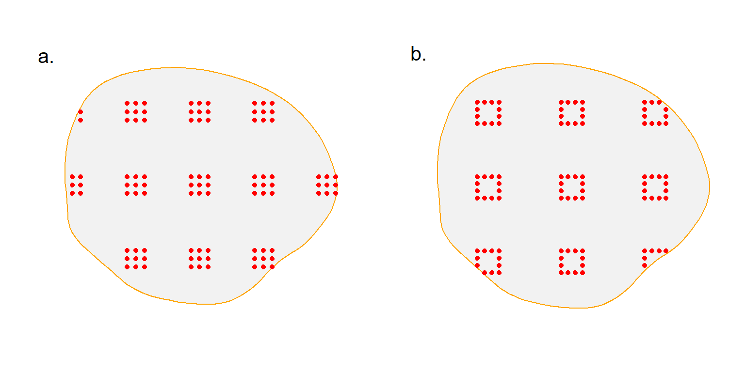
Random systematic designs usually provide a representative sample with lower sampling variance than a simple random sample (Cochran, 1977; Thompson, 2012). Any systematic design should have a random origin. For SECR each point on the systematic grid is the location of a subgrid. Subgrids may be any shape. We focus on square and hollow grids (Fig. 8.8), but circles, hexagons, and straight lines are also possible.
If subgrids are far apart then few individuals will be caught on more than one subgrid, and they can be designed and analysed as independent units (e.g., Clark, 2019). For design this means that the spacing of detectors on each subgrid should be optimised according to the considerations already raised in Section 8.5 to Section 8.9. For analysis it means that a homogeneous density model may be fitted to aggregated (‘mashed’) data from j subgrids as if they were collected from a single subgrid with the shared geometry and j times the density.
Truncation of subgrids at the edge of the region of interest reduces the size and value of marginal clusters. Two other geometrical designs avoid this problem: a lacework design (available in Efford (2025)) and a spatial coverage design, following Walvoort et al. (2010).
Lacework
In a lacework design, detectors are placed along two sets of equally spaced lines that cross at right angles to form a lattice (Fig. 8.9). By making the spacing of the lattice lines (lattice spacing a) an integer multiple of the spacing of detectors along lines (detector spacing b) we avoid odd spacing at the intersections. The expected number of points on a lacework design is given by E(K) = A/a2 (2a/b - 1).
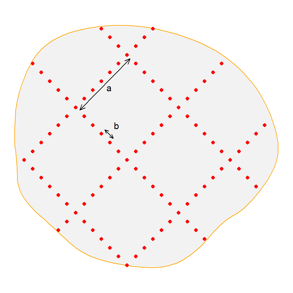
As with any systematic layout, it is desirable to randomize the origin of the lacework. The orientation is arbitrary. Lacework designs have the advantage of requiring only two design variables (a,b) when subgrid methods involve three (number or spacing of subgrids, plus spacing and extent of each subgrid).
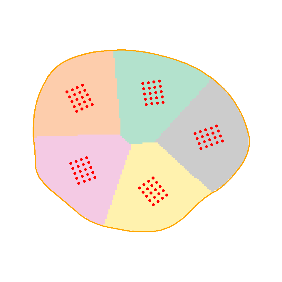
Spatial coverage
Spatial coverage may be achieved by first dividing the region of interest into equal-sized strata and then placing a subgrid in each stratum. A k-means algorithm is used to form the strata as compact clusters of pixels (Walvoort et al., 2010). A detector cluster may be centred or placed at random within each stratum (Fig. 8.10). We include the spatial coverage approach here because it uses nested subgrids, although the result is not strictly systematic.
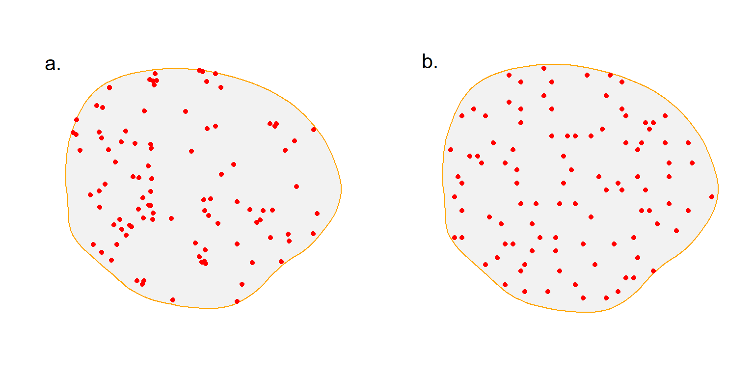
8.12.3 Non-systematic designs
Non-systematic designs result from algorithms for the placement of detectors that do not impose a particular geometry. One candidate is a simple random sample of points in the region of interest (SRS). Various algorithms improve on SRS with respect to spatial balance and efficiency. We focus on the Generalized Random Tessellation Stratified algorithm implemented by Dumelle et al. (2023) in the R package spsurvey, but there are other options (Robertson et al., 2018).
Algorithmic optimisation
Choosing a set of detector locations may be reduced to finding a subset of potential locations that maximises some criterion (benefit function). A genetic algorithm is a robust way to search the vast set of possible layouts. Wolters (2015) implemented a genetic algorithm in R that was subsequently applied to the optimisation of SECR designs by Dupont et al. (2021) and Durbach et al. (2021). The set of potential locations may simply be a fine grid of points, excluding points that are deemed inaccessible or fall in non-habitat. Results depend on the choice of criterion: Durbach et al. (2021) used the minimum of E(n) and E(r), following the suggestion of Efford & Boulanger (2019) that this often leads to near-maximal precision of \hat D. Optimisation may take many iterations and results are not unique.
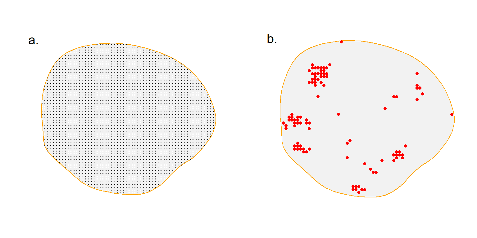
A larger criticism is that the resulting layouts are not spatially representative. The example in Fig. 8.11 shows 100 detectors placed “optimally” when RK = 0.16. Detectors are clumped to maximise the precision criterion min(E(n), E(r)) without regard to spatial balance. We view this to be a major weakness and discourage general use of the method except for exploratory purposes.
Algorithmic optimisation has revealed one point that makes intuitive sense and is otherwise hidden. AC near the edge tend to have access to fewer detectors than central AC, and increased density of detectors near the edge is beneficial for increasing n, but may reduce r (Dupont et al., 2021).
8.12.4 Comparison of clustered layouts
There is no general way to navigate the multiplicity of clustered designs. As an example, we compare the preceding clustered designs for a particular scenario: 100 binary proximity detectors in a 1-km2 region of interest for a species with \sigma = 0.02 km (RK = 0.16) keeping other parameters as in Fig. 8.5.
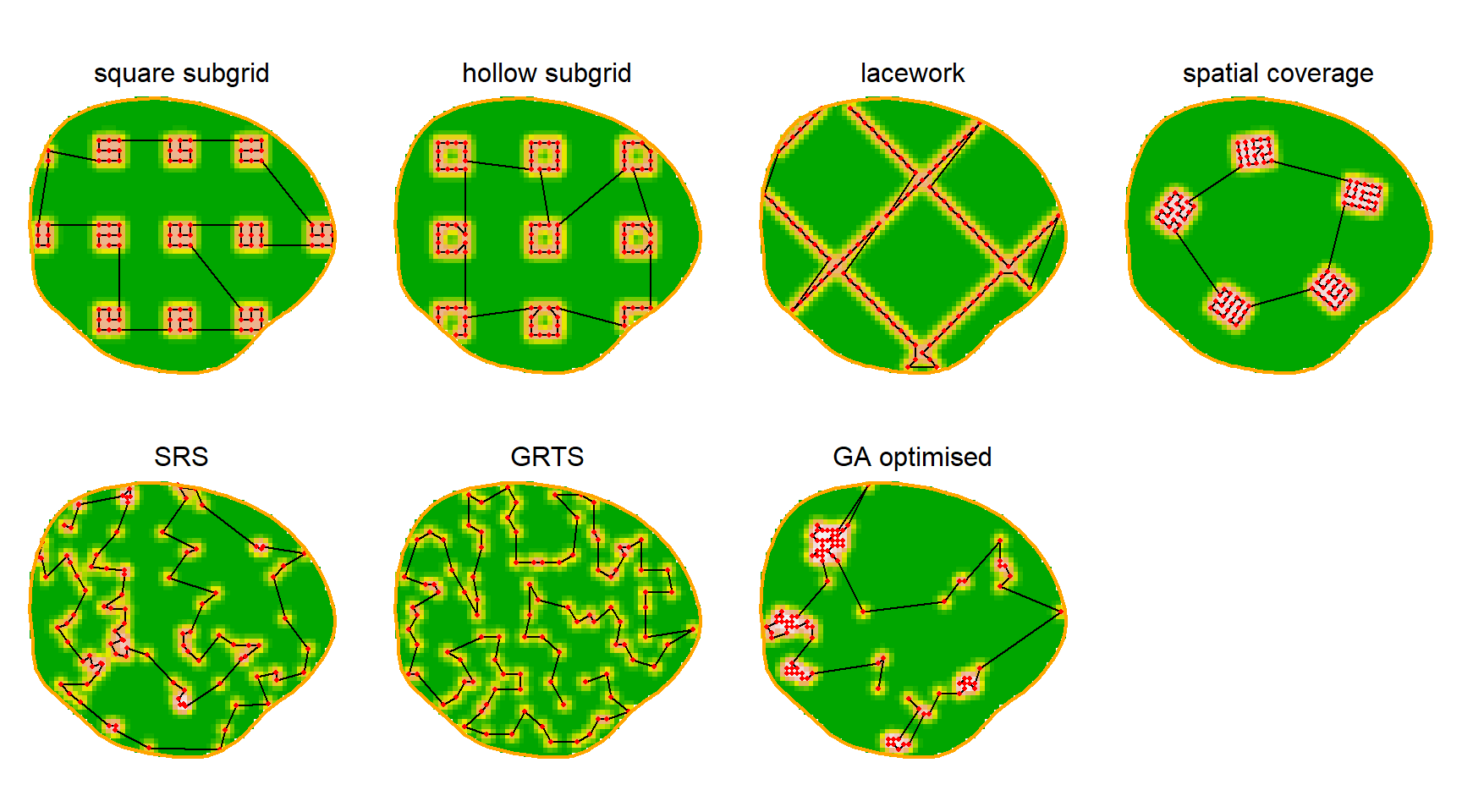
As before, we expected precision to be driven by sample size, n and r, with E(n) maximised by scattering detectors widely. Differences among the designs with respect to the usual measures of performance (RB, RSE, rRMSE) were mostly minor (Table 8.1). The exceptions were SRS (\mathrm{RB}(\hat D) +4%) and GRTS (\mathrm{RB}(\hat D) +5%); these designs detected many individuals, but generated few re-detections. The lacework design gave similar results to SRS in this instance, but results can be improved with closer spacing along fewer lines.
The algorithmically optimised design was one of several with \mathrm{RSE}(\hat D) \approx 11\%. Tight clustering of detectors resulted in the shortest travel distance of the designs considered. However, ‘GA optimised’ clearly lacked spatial balance and is therefore likely to provide biased estimates of average density if density varies systematically across the region.
Costing is complex and study-specific. Travel is an important component (time or mileage) and so we computed the length of the shortest route that included all detectors. Other components are the cost of detectors and initial setup (both proportional to K), and laboratory processing of DNA samples (proportional to n+r. Optimal route length is an example of the ‘traveling salesman problem’ (TSP). Heuristic methods in R package TSP (Hahsler & Hornik, 2007) do not produce a single minimum and perform poorly with regular grids. We therefore used the Concorde software outside R to obtain optimal routes.
| Design | K | E(n) | E(r) | E(m) | RB | RSE | rRMSE | L km |
|---|---|---|---|---|---|---|---|---|
| square subgrid | 98 | 191 | 101 | 54 | 0.6 | 10.6 | 9.7 | 6.2 |
| hollow subgrid | 99 | 196 | 99 | 52 | 0.2 | 11.2 | 9.5 | 5.5 |
| lacework | 103 | 217 | 93 | 41 | 1.2 | 11.7 | 11.9 | 5.4 |
| spatial coverage | 100 | 182 | 124 | 74 | 1.0 | 9.4 | 10.0 | 5.9 |
| SRS | 100 | 215 | 92 | 39 | 1.5 | 14.2 | 14.9 | 7.2 |
| GRTS | 100 | 239 | 68 | 12 | 2.2 | 17.1 | 23.3 | 8.1 |
| GA optimised | 100 | 153 | 153 | 112 | 1.0 | 10.6 | 10.3 | 5.2 |
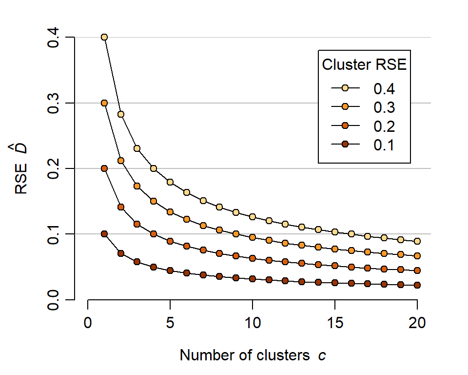
8.13 How many clusters?
For the preceding comparison we fixed the number of detectors in advance. More realistically, we might set a target \mathrm{RSE}(\hat D) and ask how many clusters (i.e. subgrids) are required. Efford & Boulanger (2019) observed that if clusters are independent (widely spaced) then E(n) and E(r) both scale with the number of clusters c, and \mathrm{RSE}(\hat D) scales with 1/ \sqrt c. Thus we can predict the precision for a single cluster and extrapolate to assemblages of clusters (Fig. 8.13). Having determined the required number of clusters we can decide on a systematic spacing or apply the spatial coverage method.
8.14 Designing for spatial variation in parameters
We have so far treated the parameters of the SECR model as constant across space. How should designs be modified to allow for spatial variation?
We must first understand the interaction between spatial variation in density and sampling intensity. Variation in density alone is not a source of significant bias in SECR. However, when sampling is more intensive in areas of high density, or areas of low density, a model that assumes homogeneous density and sampling produces biased estimates.
Some aspects of sampling intensity are under the control of the experimenter: these are the type, number and spacing of detectors, and the duration of sampling. We group these under the heading ‘sampling effort’. They will usually be known and included explicitly in the SECR model.
Other variation in sampling intensity may be due to behavioural or habitat factors that drive spatial variation in detection parameters (e.g., \lambda_0, \sigma) unknown to the experimenter.
We illustrate six scenarios for the interaction between spatial variation in density and effort, and between density and detection in Fig. 8.14. The estimate of overall density (\hat D from the null model D \sim 1) is unbiased when effort and detection are homogeneous (Fig. 8.14 a,d). Uncorrelated variation in effort does not bias \hat D (Fig. 8.14 b).
Selectively reducing effort in low-density areas (Fig. 8.14 c) causes significant bias that may be reduced or eliminated by modelling the variation in density. In the simple scenario of Fig. 8.14 c, a binary variable ‘habitat’ distinguishing between known low-density and high-density areas could be used in a model (D \sim habitat).
Variation in detection parameters causes bias even when not correlated with density (Fig. 8.14 e). This is the effect of inhomogeneous detection noted previously. The effect is large when density and detection are correlated (Fig. 8.14 f and McLellan et al. (2023)).
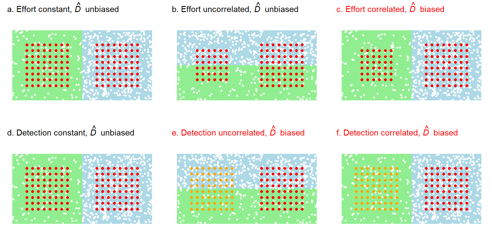
Spatially representative sampling aims to avoid correlation between density and effort (Fig. 8.14 c). A strong spatial model for density overcomes the problem, but it cannot usually be guaranteed that suitable covariates will be found, and representative sampling insures against model failure.
Stratified sampling
Deliberate stratification of effort is a special case. Stratification is used in conventional sampling to increase the precision of estimates for a given effort (e.g., Cochran, 1977; Thompson, 2012). We note that in SECR only detected individuals and their re-detections contribute to the estimation of detection parameters and, in this respect, effort in low-density areas is mostly wasted. Greater precision may therefore be achieved in some studies by concentrating effort where high density is expected. This requires care. A stratified analysis combines stratum-specific density estimates as follows.
Suppose a region of interest with area A may be divided into H subregions with area A_h where A = \sum_h A_h. Subregions have densities D_1, D_2, ..., D_H. Independent SECR sampling followed by separate model fitting in each region provides estimates \hat D_1, \hat D_2, ..., \hat D_H. The weight for each region is based on its area: W_h = A_h/A and \sum_h W_h = 1.
Then an estimate of overall density is \hat D = \sum_h W_h \hat D_h and an estimate of the sampling variance is \widehat {\mathrm{var}} (\hat D) = \sum_{h=1}^H W_h^2 \widehat {\mathrm{var}} (D_h).
The benefits of stratification for SECR have yet to be fully analysed. They are likely to be greatest when strata of contrasting density are easily distinguished, and when uncertainty regarding detection parameters (and hence the effective sampling area) dominates \mathrm{var}(n) = s^2 in the combined variance.
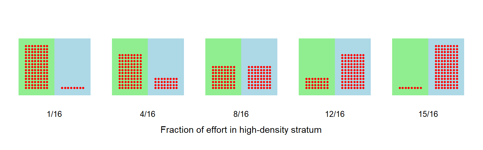
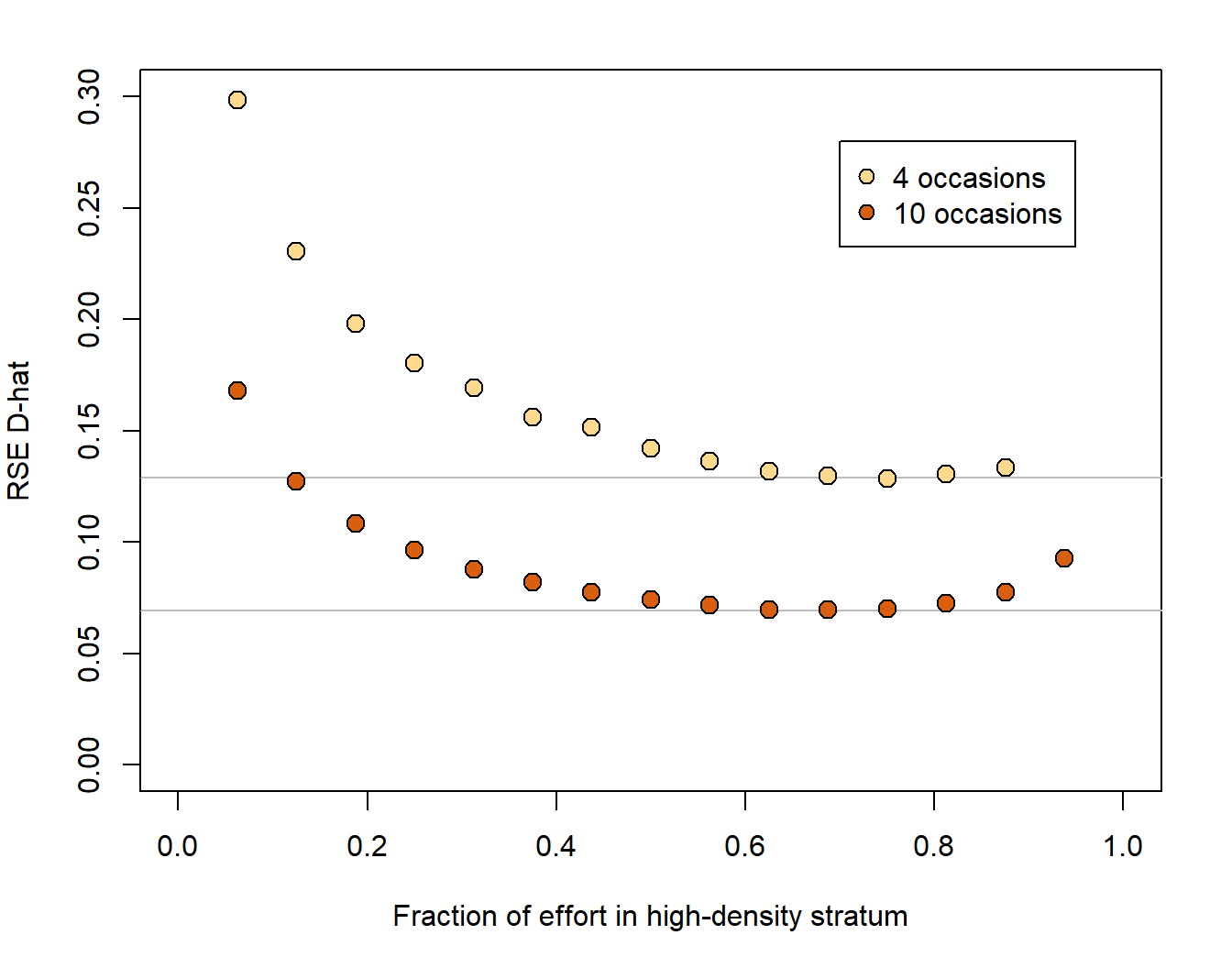
We conducted a simulation experiment with two density strata (40% and 160% of the overall average) and a constant total effort allocated differentially (Fig. 8.15). Details are on GitHub. For this example precision was best when about 70% of detectors were placed in the high-density stratum, but the improvement over equal allocation was tiny (\Delta\mathrm{RSE} \approx 0.005) for 10 occasions and small (\Delta\mathrm{RSE} \approx 0.013) for 4 occasions. Effort may also be stratified by varying the number of sampling occasions.
It may help to assume that detection parameters are uniform throughout (i.e. shared among strata); a formal test of detection homogeneity is likely to have low power.
8.15 Summary
The SECR method is very flexible, within limits. Our approach to study design for SECR is not prescriptive. Users should bear in mind these principles:
- sampling should be representative of the area of interest
- without large samples a study may lack the statistical power to answer real-world questions (this is not unique to SECR)
- two scales are important - the size of the area of interest and the scale of movement/detection
- robustness to model misspecification is greatest when the detector array spans several home ranges (Fig. 8.4)
- precise estimation of density requires both many individuals (n) and many recaptures (r) and these aspects of sample size often entail a design tradeoff
- large areas may be sampled with clustered detectors in various configurations
- logistic feasibility and cost considerations may override power in deciding among designs
- unmodelled spatial heterogeneity of density is not problematic in itself, but becomes so when confounded with spatially heterogeneous detection, due either to known variation in effort or to unseen factors
- stratified sampling (concentrating sampling effort where density is predicted to be greater) has the potential to increase precision, but in our exploratory simulation the gains were minimal.
It should be stressed that our simulation results (e.g., Fig. 8.4, Fig. 8.6, Fig. 8.7, Fig. 8.16, and Table 8.1) relate to particular scenarios, and the conclusions we draw may be reversed in other scenarios.
More generally, \sigma = \sqrt \frac{a}{\pi \log [(1-p)^{-2}]} where p is the probability contour (Jennrich & Turner, 1969 Eq. 12).↩︎