Appendix H — Parameterizations

At the heart of SECR there is usually a set of three primary model parameters: one for population density ( $D$ ) and two for the detection function. The detection function is commonly parameterized in terms of its intercept (the probability $g_0$ or cumulative hazard $\lambda_0$ of detection for a detector at the centre of the home range) and a spatial scale parameter $\sigma$ . Although this parameterization is simple and uncontroversial, it is not inevitable. Sometimes the biology leads us to expect a structural relationship between primary parameters. The relationship may be ‘hard-wired’ into the model by replacing a primary parameter with a function of other parameter(s). This often makes for a more parsimonious model, and model comparisons may be used to evaluate the hypothesized relationship. Here we outline some parameterization options in secr.

H.1 Theory

The idea is to replace a primary detection parameter with a function of other parameter(s) in the SECR model. This may allow constraints to be applied more meaningfully. Specifically, it may make sense to consider a function of the parameters to be constant, even when one of the primary parameters varies. The new parameter also may be modelled as a function of covariates etc.

H.1.1 $\lambda_0$ and $\sigma$

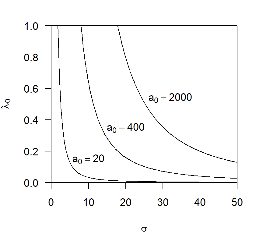
One published example concerns compensatory heterogeneity of detection parameters (Efford and Mowat 2014). Combinations of $\lambda_0$ and $\sigma$ yield the same effective sampling area $a$ when the cumulative hazard of detection ( $\lambda(d)$ )¹ is a linear function of home-range utilisation. Variation in home-range size then has no effect on estimates of density. It would be useful to allow $\sigma$ to vary while holding $a$ constant, but this has some fishhooks because computation of $\lambda_0$ from $a$ and $\sigma$ is not straightforward. A simple alternative is to substitute $a_0 = 2 \pi \lambda_0 \sigma^2$ ; Efford & Mowat (2014) called $a_0$ the ‘single-detector sampling area’. If the sampling regime is constant, holding $a_0$ constant is almost equivalent to holding $a$ constant (but see Limitations). Fig. H.1 illustrates the relationship for 3 levels of $a_0$ .

Figure H.1: Structural relationship between parameters $\lambda_0$ and $\sigma$ expressed by holding $a_0$ constant in $\lambda_0 = a_0 / (2 \pi \sigma^2)$ .

H.1.2 $\sigma$ and $D$

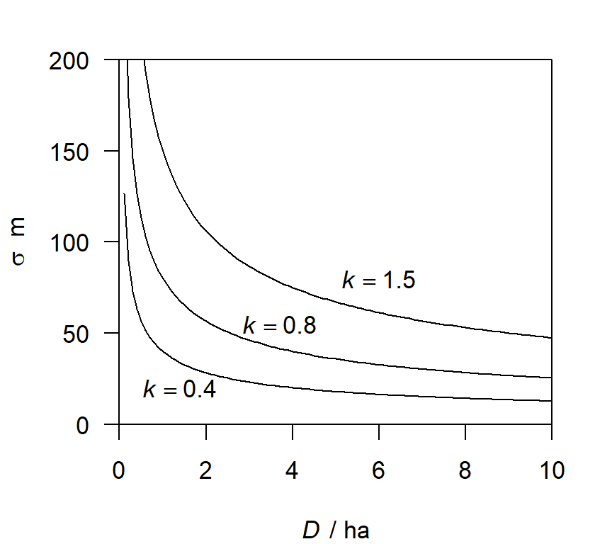
Another biologically interesting structural relationship is that between population density and home-range size (Efford et al., 2016). If home ranges have a definite edge and partition all available space then an inverse-square relationship is expected $D = (k / r)^2$ or $r = k / \sqrt D$ , where $r$ is a linear measure of home-range size (e.g., grid cell width) and $k$ is a constant of proportionality. In reality, the home-range model that underlies SECR detection functions does not require a hard edge, so the language of ‘partitioning’ and ‘elastic discs’ (Huxley, 1934) does not quite fit. However, the inverse-square relationship is empirically useful, and we conjecture that it may also arise from simple models for constant overlap of home ranges when density varies – a topic for future research. For use in SECR we equate $r$ with the spatial scale of detection $\sigma$ , and predict concave-up relationships as in Fig. H.2.

The relationship may be modified by adding a constant $c$ to represent the lower asymptote of sigma as density increases ( $\sigma = k / \sqrt D + c$ ; by default $c = 0$ in secr).

It is possible, intuitively, that once a population becomes very sparse there is no further effect of density on home-range size. Alternatively, very low density may reflect sparseness of resources, requiring the few individuals present to exploit very large home ranges even if they seldom meet. If density is no longer related to $\sigma$ at low density, even indirectly, then the steep increase in $\sigma$ modelled on the left of Fig. H.3 will ‘level off’ at some value of $\sigma$ . We don’t know of any empirical example of this hypothetical phenomenon, and do not provide a model.

Figure H.2: Structural relationship between parameters $D$ and $\sigma$ expressed by holding $k$ constant in $\sigma = 100 k / \sqrt D$ . The factor of 100 adjusts for the inconsistent default units of $\sigma$ and $D$ in **secr** (metres and hectares).

We use ‘primary parameter’ to mean one of ( $D, \lambda_0, \sigma$ )² For each relationship there is a primary parameter considered the ‘driver’ that varies for external reasons (e.g., between times, sexes etc.), and a dependent parameter that varies in response to the driver, moderated by a ‘surrogate’ parameter that may be constant or under external control. The surrogate parameter appears in the model in place of the dependent parameter. Using the surrogate parameterization is exactly equivalent to the default parameterization if the driver parameter(s) ( $\sigma$ and $\lambda_0$ for $a_0$ ³, $D$ for $k$ ⁴) are constant.

H.2 Implementation

Parameterizations in secr are indicated by an integer code (Table H.1). The internal implementation of the parameterizations (3)–(5) is straightforward. At each evaluation of the likelihood function:

The values of the driver and surrogate parameters are determined
Each dependent parameter is computed from the relevant driver and surrogate parameters
Values of the now-complete set of primary parameters are passed to the standard code for evaluating the likelihood.

Table H.1: Parameterization codes.

Code	Description	Driver	Surrogate(s)	Dependent
0	Default	–	–	–
3	Single-detector sampling area	$\sigma$	$a_0$	$\lambda_0 = a_0/(2\pi\sigma^2)$
4	Density-dependent home range	$D$	$k$ , $c$	$\sigma = 100 k / \sqrt D + c$
5	3 & 4 combined	$D$ , $\sigma$	$k$ , $c$ , $a_0$	$\sigma = 100 k / \sqrt D + c$ , $\lambda_0 = a_0/(2\pi\sigma^2)$

The transformation is performed independently for each level of the surrogate parameters that appears in the model. For example, if the model includes a learned response a0 ~ b, there are two levels of a0 (for naive and experienced animals) that translate to two levels of lambda0. For parameterization (4), $\sigma = 100 k / \sqrt D$ . The factor of 100 is an adjustment for differing units (areas are expressed in hectares in secr, and 1 hectare = 10 000 $\mathrm{m}^2$ ). For parameterization (5), $\sigma$ is first computed from $D$ , and then $\lambda_0$ is computed from $\sigma$ .

H.2.1 Interface

Users choose between parameterizations either

explicitly, by setting the ‘param’ component of the secr.fit argument ‘details’, or
implicitly, by including a parameterization-specific parameter name in the secr.fit model.

Implicit selection causes the value of details$param to be set automatically (with a warning).

The main parameterization options are listed in Table 1 (other specialised options are listed in Section H.5).

The constant $c$ in the relationship $\sigma = k / \sqrt{D} + c$ is set to zero and not estimated unless ‘c’ appears explicitly in the model. For example, model = list(sigmak ~ 1) fixes c = 0, whereas model = list(sigmak ~ 1, c ~ 1) causes c to be estimated. The usefulness of this model has yet to be proven! By default an identity link is used for ‘c’, which permits negative values; negative ‘c’ implies that for some densities (most likely densities outside the range of the data) a negative sigma is predicted. If you’re uncomfortable with this and require ‘c’ to be positive then set link = list(c = 'log') in secr.fit and specify a positive starting value for it in start (using the vector form for that argument of secr.fit).

Initial values may be a problem as the scales for a0 and sigmak are not intuitive. Assuming automatic initial values can be computed for a half-normal detection function with parameters $g_0$ and $\sigma$ , the default initial value for $a_0$ is $2 \pi g_0 \sigma^2 /10000$ , and for $k$ , $\sigma \sqrt{D}$ . If the usual automatic procedure (see ?autoini) fails then ad hoc and less reliable starting values are used. In case of trouble, it is suggested that you first fit a very simple (or null) model using the desired parameterization, and then use this to provide starting values for a more complex model. Here is an example (actually a trivial one for which the default starting values would have been OK; some warnings are suppressed):

fit0  <- secr.fit(captdata, model = a0~1, detectfn = 'HHN',
                  trace = FALSE)
fitbk <- secr.fit(captdata, model = a0~bk, detectfn = 'HHN', 
                  trace = FALSE, start = fit0)

H.2.2 Models for surrogate parameters a0 and sigmak

The surrogate parameters a0 and sigmak are treated as if they are full ‘real’ parameters, so they appear in the output from predict.secr, and may be modelled like any other ‘real’ parameter. For example, model = sigmak ~ h2 is valid.

Do not confuse this with the modelling of primary ‘real’ parameters as functions of covariates, or built-in effects such as a learned response.

H.3 Example

Among the datasets included with secr, only ovenCH provides a useful temporal sequence - 5 years of data from mistnetting of ovenbirds (Seiurus aurocapilla) at Patuxent Research Refuge, Maryland. A full model for annually varying density and detection parameters may be fitted with

msk <- make.mask(traps(ovenCH[[1]]), buffer = 300, nx = 25)
oven0509b <- secr.fit(ovenCH, model = list(D ~ session, 
    sigma ~ session, lambda0 ~ session + bk), mask = msk, 
    detectfn = 'HHN', trace = FALSE)

This has 16 parameters and takes some time to fit.

We hypothesize that home-range (territory) size varied inversely with density, and model this by fixing the parameter $k$ . Efford & Mowat (2014) reported for this dataset that $\lambda_0$ did not compensate for within-year, between-individual variation in $\sigma$ , but it is nevertheless possible that variation between years was compensatory, and we model this by fixing $a_0$ . For good measure, we also allow for site-specific net shyness by modelling $a_0$ with the builtin effect ‘bk’:

oven0509bs <- secr.fit(ovenCH, model = list(D ~ session, sigmak ~ 1,
    a0 ~ bk), mask = msk, detectfn = 'HHN', trace = FALSE)

Warning: Using parameterization details$param = 5

The effect of including both sigmak and a0 in the model is to force parameterization (5). The model estimates a different density in each year, as in the previous model. Annual variation in $D$ drives annual variation in $\sigma$ through the relation $\sigma_y = k / \sqrt{D_y}$ where $k$ (= sigmak/100) is a parameter to be estimated and the subscript $y$ indicates year. The detection function ‘HHN’ is the hazard-half-normal which has parameters $\sigma$ and $\lambda_0$ . We already have year-specific $\sigma_y$ , and this drives annual variation in $\lambda_0$ : $\lambda_{0y} = a_{0X} / (2 \pi \sigma_y^2)$ where $a_{0X}$ takes one of two different values depending on whether the bird in question has been caught previously in this net.

This is a behaviourally plausible and fairly complex model, but it uses just 8 parameters compared to 16 in a full annual model with net shyness. It may be compared by AIC with the full model (the model structure differs but the data are the same). Although the new model has somewhat higher deviance (1858.5 vs 1851.6), the reduced number of parameters results in a substantially lower AIC ( $\Delta$ AIC = 9.1).

In Fig. H.3 we illustrate the results by overplotting the fitted curve for $\sigma_y$ on a scatter plot of the separate annual estimates from the full model. A longer run of years was analysed by Efford et al. (2016).

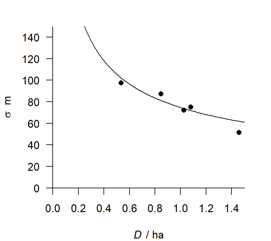
Figure H.3: Fitted structural relationship between parameters $D$ and $\sigma$ (curve; $\hat k =$ `r round(predict(oven0509bs)[[1]]['sigmak','estimate']/100,3)`) and separate annual estimates (ovenbirds mistnetted on Patuxent Research Refuge 2005–2009).

H.4 Limitations

Using $a_0$ as a surrogate for $a$ is unreliable if the distribution or intensity of sampling varies. This is because $a_0$ depends only on the parameter values, whereas $a$ depends also on the detector layout and duration of sampling. For example, if a different size of trapping grid is used in each session, $a$ will vary even if the detection parameters, and hence $a_0$ , stay the same. This is also true ( $a$ varies, $a_0$ constant) if the same trapping grid is operated for differing number of occasions in each session. It is $a$ that really matters, and constant $a_0$ is not a sensible null model in these scenarios.

parameterizations (4) and (5) make sense only if density D is in the model; an attempt to use these when maximizing only the conditional likelihood (CL = TRUE) will cause an error.

H.5 Other notes

Detection functions 0–3 and 5–8 (‘HN’,‘HR’,‘EX’, ‘CHN’, ‘WEX’, ‘ANN’, ‘CLN’, ‘CG’) describe the probability of detection $g(d)$ and use $g_0$ as the intercept instead of $\lambda_0$ . Can parameterizations (3) and (5) also be used with these detection functions? Yes, but the user must take responsibility for the interpretation, which is less clear than for detection functions based on the cumulative hazard (14–19, or ‘HHN’, ‘HHR’, ‘HEX’, ‘HAN’, ‘HCG’, ‘HVP’). The primary parameter is computed as $g_0 = 1 - \exp(-a_0 / (2\pi \sigma^2))$ .

In a sense, the choice between detection functions ‘HN’ and ‘HHN’, ‘EX’ and ‘HEX’ etc. is between two parameterizations, one with half-normal hazard $\lambda(d)$ and one with half-normal probability $g(d)$ , always with the relationship $g(d) = 1 - \exp(-\lambda(d))$ (using $d$ for the distance between home-range centre and detector). It may have been clearer if this had been programmed originally as a switch between ‘hazard’ and ‘probability’ parameterizations, but this would now require significant changes to the code and is not a priority.

If a detection function is specified that requires a third parameter (e.g., z in the case of the hazard-rate function ‘HR’) then this is carried along untouched.

It is possible that home range size, and hence $\sigma$ , varies in a spatially continuous way with density. The sigmak parameterization does not work when density varies spatially within one population because of the way models of state variables ( $D$ ) and detection variables ( $g_0$ , $\lambda_0$ , $\sigma$ ) are separated within secr. Non-Euclidean distance methods allow a workaround as described in Appendix F and Efford et al. (2016).

Some parameterization options (Table H.2) were not included in Table H.1 because they are not intended for general use and their implementation may be incomplete (e.g., not allowing covariates). Although parameterizations (2) and (6) promise a ‘pure’ implementation in terms of the effective sampling area $a$ rather than the surrogate $a_0$ , this option has not been implemented and tested as extensively as that for $a_0$ (parameterization 3). The transformation to determine $\lambda_0$ or $g_0$ requires numerical root finding, which is slow. Also, assuming constant $a$ does not make sense when either the detector array or the number of sampling occasions varies, as both of these must affect $a$ . Use at your own risk!

Table H.2: Additional parameterizations.

Code	Description	Driver	Surrogate(s)	Dependent
2	Effective sampling area	$\sigma$	$a$	$\lambda_0$ such that $a = \int p_\cdot(\mathbf x\|\sigma, \lambda_0) d\mathbf x$
6	2 & 4 combined	$D$	$k$ , $c$ , $a$	$\sigma = 100 k / \sqrt D + c$ , $\lambda_0$ as above

H.6 Abundance

We use density $D$ as the primary parameter for abundance; the number of activity centres $N(A)$ is secondary as it is contingent on delineation of an area $A$ .

Appendix J considers an alternative parameterization of multi-session density in terms of the initial density $D_1$ and session-to-session trend $\lambda_t$ .

The cumulative hazard $\lambda(d)$ and probability $g(d)$ formulations are largely interchangeable because $g(d) = 1 - \exp(-\lambda(d))$ .↩︎
secr names D, lambda0 or sigma.↩︎
secr name a0↩︎
secr uses sigmak = $100k$ ↩︎