17 Simulation
Simulation has many uses in SECR; we focus particularly on
- determining properties of estimators under breaches of assumptions (Chapter 6),
- assessing candidate study designs (Chapter 8), and
- assessing goodness of fit (Chapter 13).
The first two of these are not related to the analysis of a dataset and the required ‘de novo’ simulations follow essentially the same steps in secr, as detailed below. The third entails simulation from a particular model fitted to data, as considered earlier. Other uses of simulation are more niche – parameter estimation (Efford, 2023), testing software implementations, and the computation of parametric bootstrap confidence intervals.
This chapter aims to demystify simulation and make it available to a wider range of SECR users. We start by breaking a simulation down into the component steps, showing how each of these may be performed in secr. Later we introduce the package secrdesign that manages these steps for greater efficiency.
17.1 Simulation step by step
The essential steps for each replicate of a de novo SECR simulation are
- Generate an instance of the population process, i.e. the distribution of activity centres AC.
- Generate a set of ‘observed’ spatial detection histories from the AC distribution according to some study design (detector layout, sampling duration), and detection parameters (e.g., \lambda_0, \sigma).
- Fit an SECR model to estimate parameters of the population and detection processes, along with their sampling variances.
It is simple enough to perform steps 1 & 2 directly in R without the use of secr functions. We give an example before describing functions that cover many variations with less code.
# Step 2a. Sample from population with central 6 x 6 detector array
detxy <- expand.grid(x = seq(100,200,20), y = seq(100,200,20))
K     <- nrow(detxy)                      # number of detectors
S     <- 5                                # number of occasions
g0    <- 0.2                              # detection parameter
sigma <- 20                               # detection parameter
d     <- secr::edist(popxy, detxy)        # distance to detectors
p     <- g0 * exp(-d^2/2/sigma^2)         # probability detected
detected <- as.numeric(runif(N*K*S) < rep(p,S))
ch    <- array(detected, dim = c(N,K,S), dimnames = list(1:N, 1:K, 1:S))
ch    <- ch[apply(ch,1,sum)>0,,]          # reject null histories

# Step 2b. Cast simulated data as an secr 'capthist' object
class(detxy)    <- c('traps', 'data.frame')
detector(detxy) <- 'proximity'
ch              <- aperm(ch, c(1,3,2))   # permute dim to N, S, K
class(ch)       <- 'capthist'
traps(ch)       <- detxy
Now that the data are in the right shape we can proceed to fit a model:
# Step 3. Fit model to simulated capthist
fit <- secr.fit(ch, buffer = 100, trace = FALSE)
predict(fit)
link estimate SE.estimate lcl ucl
D log 18.53043 2.7611 13.85955 24.77548
g0 logit 0.22101 0.0235 0.17838 0.27046
sigma log 20.11668 1.0532 18.15608 22.28900This is rather laborious and it’s easy to slip up. We next outline the secr functions sim.popn and sim.capthist that conveniently wrap Steps 1 & 2, respectively, along with many extensions.
A further level of wrapping is provided by package secrdesign that manages simulation scenarios, their replicated execution (Steps 1–3), and the summarisation of results.
17.1.1 Simulating AC distributions with sim.popn
A simulated AC distribution is an object of class ‘popn’ in secr. This is usually a distribution of points within a rectangular region that is the bounding box of a ‘core’ object (most likely a ‘traps’ object) inflated by a certain ‘buffer’ distance in metres. sim.popn generates a ‘popn’ object, for which there is a plot method.
tr <- make.grid()  # a traps object, for demonstration
pop <- sim.popn(D = 10, core = tr, buffer = 100,
    model2D = "poisson")
par(mar = c(1,1,1,1))
plot(pop)
plot(tr, add = TRUE)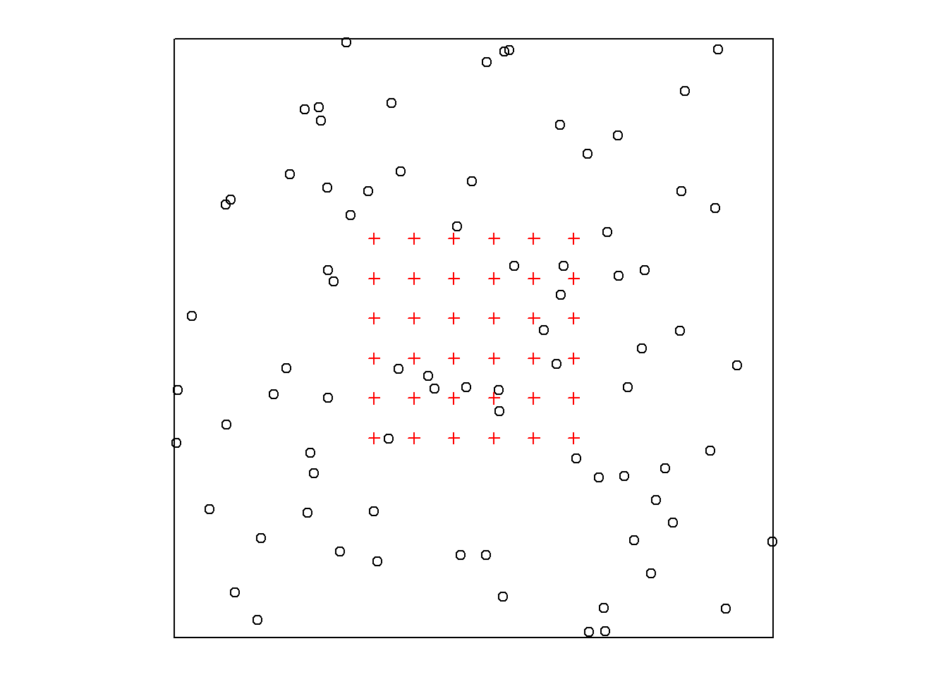
The default 2-D distribution is random uniform - a Poisson distribution, as shown here. The expected number of activity centres E(NA) is determined by the argument D, the density in AC per hectare. By default NA is a Poisson random variable, but it may be fixed by setting Ndist = "fixed". Published simulations often fix NA for reasons of convenience such as avoiding realisations that may be hard to model or reducing the variance among replicates. Comparisons must therefore be made with care.
For Ndist = "poisson" the choice of buffer is not critical so long as it is large enough to include all potentially detected AC. Simulated populations with excessively large NA take longer to sample (the next step - generating a capthist object), but the ultimate capthist is no larger and model fitting takes the same time.
Inhomogeneous alternatives to a uniform random distribution may be specified using the arguments ‘model2D’ and ‘details’. We elaborate on these later.
17.1.2 Simulating detection with sim.capthist
To simulate sampling of a given population we specify the type and spatial distribution of detectors, the detection function, and the duration of sampling. Detectors are prepared in advance as an object of class ‘traps’, either input from a data file or generated by one of the functions for a specific geometry (make.grid, trap.builder, make.systematic, make.circle etc.).
ch <- sim.capthist(traps = tr, popn = pop, detectpar = list(
    g0 = 0.1, sigma = 20), noccasions = 5, renumber = FALSE)
summary(ch)
Object class capthist
Detector type multi (5)
Detector number 36
Average spacing 20 m
x-range 0 100 m
y-range 0 100 m
Counts by occasion
1 2 3 4 5 Total
n 10 7 9 5 7 38
u 10 7 0 0 1 18
f 5 8 3 2 0 18
M(t+1) 10 17 17 17 18 18
losses 0 0 0 0 0 0
detections 10 7 9 5 7 38
detectors visited 10 7 7 5 6 35
detectors used 36 36 36 36 36 180
Individual covariates
sex
F:9
M:9 par(mar = c(1,1,1,1))
plot(ch, tracks = TRUE, rad = 3)
plot(pop, add = TRUE)
captured <- subset(pop, rownames(pop) %in% rownames(ch))
plot(captured, pch = 16, add = TRUE)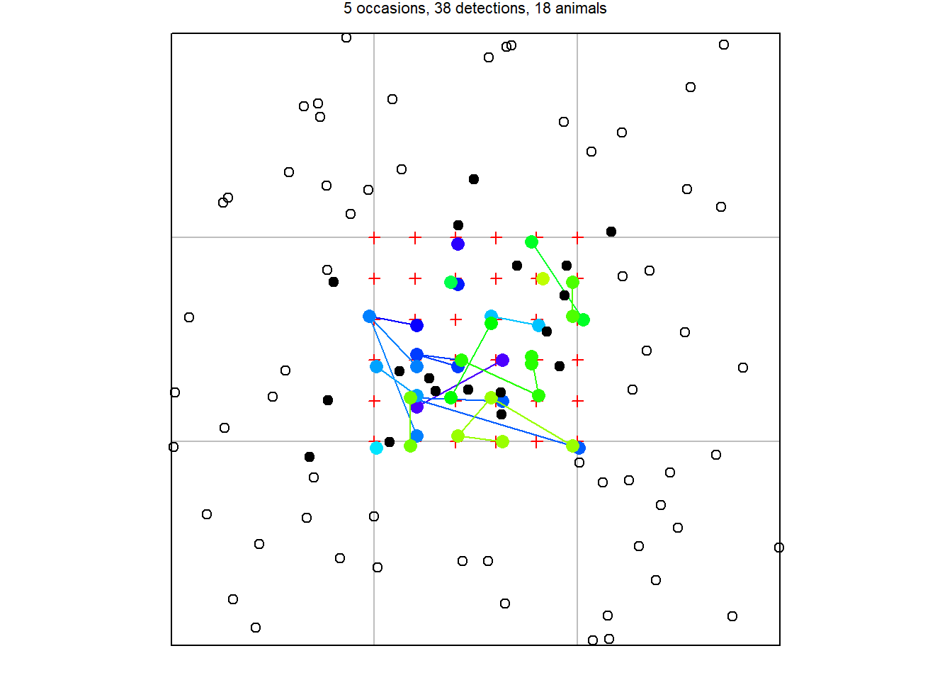
17.1.3 Combining data generation and model fitting
We loop over the AC-generation, sampling, and model-fitting steps, recording the results for later.
tr <- make.grid()  # a traps object
nrepl <- 10
set.seed(123)
out <- list()
for (r in 1:nrepl) {
    pop <- sim.popn(D = 20, core = tr, buffer = 100,
        model2D = "poisson")
    ch <- sim.capthist(traps = tr, popn = pop, detectpar = list(
        g0 = 0.2, sigma = 20), noccasions = 5)
    fit <- secr.fit(ch, buffer=100, trace = FALSE)
    out[[r]] <- predict(fit)
}
Each output returned by the predict method is a dataframe from which we extract the density estimate and its standard error to form the summary:
trueD  <- 20
Dhat   <- sapply(out, '[', 'D', 'estimate')
seDhat <- sapply(out, '[', 'D', 'SE.estimate')
cat ("mean  ", mean(Dhat), '\n')
cat ("RB    ", (mean(Dhat)-trueD) / trueD, '\n')
cat ("RSE   ", mean(seDhat / Dhat), '\n')
cat ("rRMSE ", sqrt(mean((Dhat-trueD)^2)) / mean(Dhat), '\n')
mean 20.52
RB 0.025987
RSE 0.15481
rRMSE 0.14281 17.2 Simulation in secrdesign
The R package secrdesign takes care of a lot of the coding needed to specify, execute and summarise SECR simulations. Full details are in its documentation, particularly secrdesign-vignette.pdf.
The heart of secrdesign is a dataframe of one or more scenarios. Usually there is one row per scenario. The scenario dataframe is constructed with make.scenarios. Some properties of scenarios, such as expected sample sizes, may be extracted without simulation using scenarioSummary. This is a good first check.
Simulations are executed with run.scenarios, with or without model fitting. The resulting object is summarised either directly (with the summary method) or after further processing to select fields and statistics. Several arguments of run.scenarios comprise lookup lists from which each scenario selects according to a numeric index field. For example, ‘trapset’ is a list of detector layouts, from which each scenario selects via its ‘trapsindex’ column. Likewise ‘pop.args’, ‘det.args’, and ‘fit.args’ are lists corresponding to the ‘popindex’, ‘detindex’ and ‘fitindex’ columns of the scenario data.frame. These optionally provide fine control of sim.popn, sim.capthist and secr.fit, respectively. The saved output may be customized via the ‘extractfn’ argument.
This small demonstration repeats the simulation in the preceding code. ‘xsigma’ specifies the buffer width as a multiple of ‘sigma’.
library(secrdesign)
tr   <- make.grid()
scen <- make.scenarios (D = 20, g0 = 0.2, sigma = 20,
    noccasions = 5)
sims <- run.scenarios(10, scen, tr, xsigma = 5, fit = TRUE,
    seed = 123)
## Completed scenario 1
## Completed in 0.044 minutes
We can get a compact summary like this:
estimateSummary(sims) scenario true.D nvalid EST seEST RB seRB RSE RMSE rRMSE COV
1 1 20 10 20.511 1.2833 0.025526 0.064167 0.15498 3.8837 0.19419 0.9The default sampling function sim.capthist is usually adequate, but an alternative may be specified via the argument ‘CH.function’.
Simulation quite often results in data that are too sparse for analysis, and other malfunctions are possible. As a user you should be on your guard for meaningless, extreme values in the estimates. The validate function provides a mechanism for filtering these out.
17.3 Advanced simulations
17.3.1 Inhomogeneous populations
Variations on a uniform distribution of AC are selected with the sim.popn argument ‘model2D’. This may be done directly, as when we first introduced sim.popn, or indirectly via the ‘pop.args’ argument of run.scenarios. While almost any process may be used to generate data, only the parameters of an inhomogeneous Poisson process may be estimated by fitting models in secr. Alternative methods are available for some other generating models (Dey et al., 2023; Stevenson et al., 2021).
We next consider three types of point process that may be used to simulate inhomogeneous distributions of activity centres in sim.popn.
17.3.1.1 Inhomogeneous Poisson Process
An inhomogeneous Poisson process (IHPP) is specified by setting ‘model2D = “IHP”’. The argument ‘core’ should be a habitat mask. Cell-specific density (expected number of individuals per hectare) may be given either in a covariate of the mask (named in argument ‘D’) or as a vector of values in argument ‘D’. The covariate option allows you to simulate from a previously fitted Dsurface (output from predictDsurface). Special cases of IHPP are provided in the ‘hills’ and ‘coastal’ options for ‘model2D’.
17.3.1.2 Cox Processes
In a Cox process the expected density surface of the IHPP varies randomly between realisations (i.e. replicates). For example, secr has the function randomDensity that may be used in sim.popn to generate a new binary density mosaic at each call (see Examples on its help page).
A flexible model for continuous variation in density is the log-Gaussian Cox Process (LGCP) (Dupont et al., 2021; Johnson et al., 2010; Efford2024?). The IHPP log-intensity surface of a LGCP is Gaussian (normally distributed) at each point, but adjacent points co-vary; autocorrelation declines with distance. The notation and parameterisation can be confusing. The term ‘Gaussian’ refers to the marginal intensity, not the autocorrelation function which is commonly exponential. The Gaussian variance is on the log scale, so even a variance as low as 1.0 indicates substantial heterogeneity. The exponential scale parameter naturally has the same units as the SECR detection function, although Dupont et al. (2021) rescaled it as 6% or 100% of the width of the study area. secr uses the function rLGCP from spatstat (Baddeley et al., 2015).
17.3.1.3 Cluster Processes
The points in a 2-D cluster process are no longer independent, as in an IHPP. Each belongs to a cluster. For the Thomas process that has been applied in SECR (e.g., Efford et al., 2009) there is a Poisson distribution of ‘parents’ and a bivariate-normal scatter of offspring points about each parent. Both the number of parents and the number of offspring per parent are Poisson variables, and hence some clusters may be empty. Thomas processes belong to the broader class of Neyman-Scott cluster processes. secr implements an interface to the function rThomas from spatstat (Baddeley et al., 2015) (‘model2D = “rThomas”’).
17.3.2 Summary of inhomogeneous options
Both Cox and cluster processes require additional parameters to be specified in the ‘details’ argument of sim.popn (Table 17.1). Fig. 17.3 provides examples.
sim.popn controlled by argument ‘model2D’ with additional parameters specified in the ‘details’ argument
| Type | model2D | details | Note |
|---|---|---|---|
| Uniform | “poisson” | — | |
| IHPP | “IHP” | — | cell densities pre-computed |
| “hills” | hills | sine-curve density in 2-D | |
| “coastal” | Beta | extreme gradients cf Fewster & Buckland (2004) | |
| Cox process | “rLGCP” | var, scale | |
| Cluster process | “rThomas” | mu, scale |
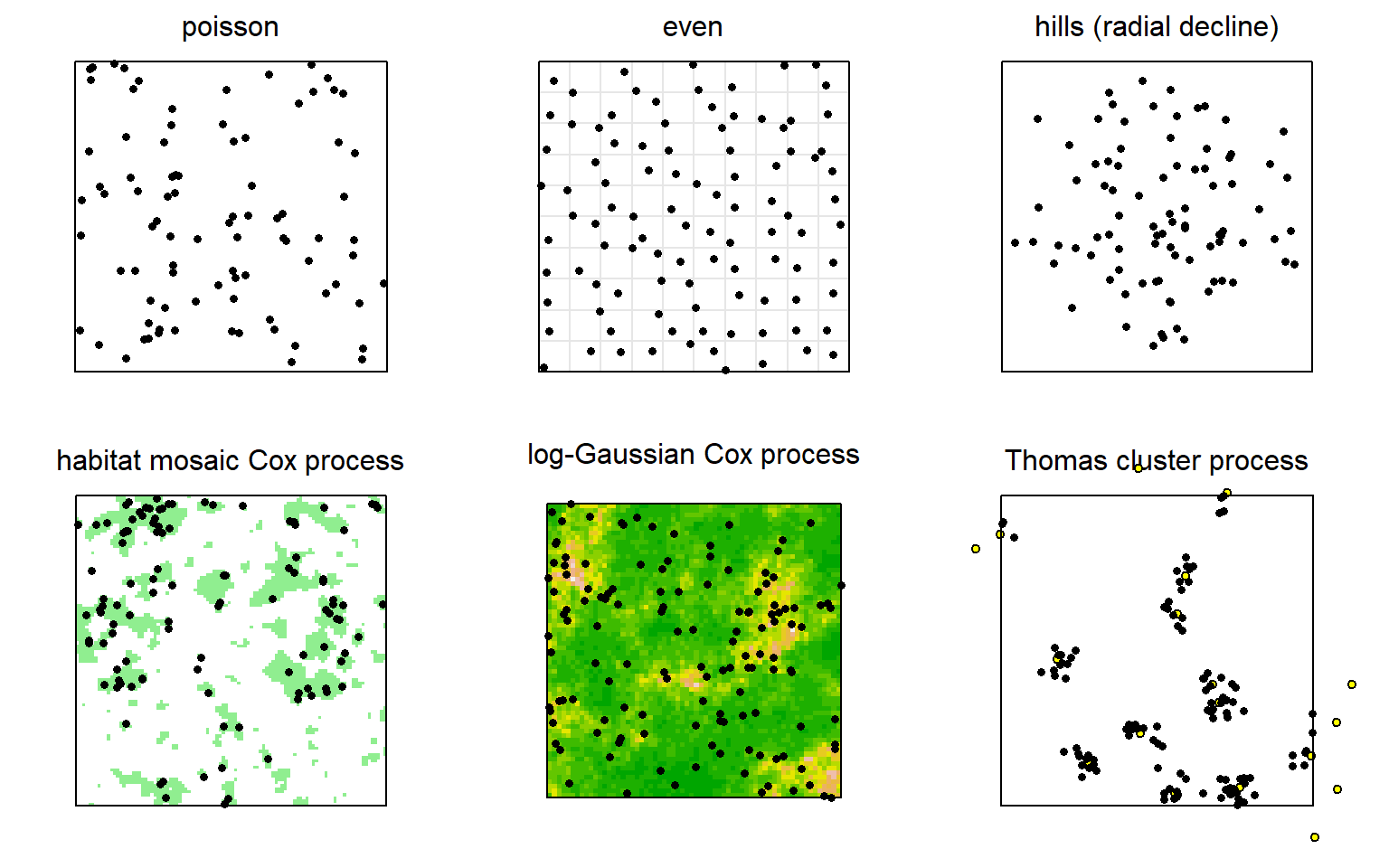
sim.popn. Yellow dots indicate location of cluster ‘parents’, some of which lie outside the frame.
17.3.3 Spatial repulsion
We can imagine scenarios in which AC are distributed more evenly than expected from a random uniform distribution, perhaps due to territorial behaviour. A point process model with repulsion between AC was considered by Reich & Gardner (2014). There is no equivalent model in sim.popn. However, the option ‘model2D = “even”’ goes some way towards it: space is divided into notional square grid cells of area 1/D and one AC is located randomly within each cell (Fig. 17.3).
17.3.4 Inhomogeneous detection
Simulating spatial variation in detection parameters is a minefield: there are many subtly different approaches and ad hoc variations (Dey et al., 2023; Efford, 2014; Hooten et al., 2024; Moqanaki et al., 2021; Royle et al., 2013; Stevenson et al., 2021).
The first question is whether to focus on the location of the detector or the location of the activity centres. We label these approaches ‘detector-centric’ and ‘AC-centric’. Focusing on detectors is simpler as they comprise a few discrete locations whereas AC are at unknown locations in continuous space.
sim.capthist allows values of g0 and lambda0 to be detector-specific. Values are provided as an occasion x detector matrix.
The authors cited at the start of this section were mainly concerned with [detector-centric] spatially auto-correlated random effects (‘SARE’, following Dey et al. (2023)). Random variation among detectors may be modelled on the link scale by a Gaussian random field. Simulation is simpler than the LGCP for AC because values are required only at the K detectors. Deviates are obtained from a random K-dimensional multivariate normal distribution with distance-dependent covariance matrix (e.g., Moqanaki et al., 2021). Simulation in secr uses custom functions, for which there are several examples on GitHub with comments on parameterisation.
A purely detector-centric approach does not allow for a model in which the activity of an individual at one point in its home range depends on resource availability both there and at other points. Normalisation of activity must then account for resource distribution in continuous space (see Efford, 2014 and the preceding GitHub site). Moqanaki et al. (2021) transformed to uniform (-1.96, 1.96)
There are more arcane options for simulating AC-centric variation in detection:
- covariates ‘lambda0’ and ‘sigma’ may be added to simulated populations on the basis of the x-y coordinates of the AC, and used in
sim.capthistby setting ‘detectpar = list(individual = TRUE)’ (requires secr \ge 4.6.7) - the ‘userdist’ argument may be used to ‘warp’ space and hence the effective sigma (cf Appendix F)
- discrete non-overlapping populations may be simulated and pasted together post hoc.