Appendix I — Density revisited

I.1 User-provided model functions

Some density models cannot be coded in the generalized linear model form of the model argument. To alleviate this problem, a model may be specified as an R function that is passed to secr.fit, specifically as the component ‘userDfn’ of the list argument ‘details’. We document this feature here, although you may never use it.

The userDfn function must follow some rules.

• It should accept four arguments, the first a vector of parameter values or a character value (below), and the second a ‘mask’ object, a data frame of x and y coordinates for points at which density must be predicted.

Argument	Description
Dbeta	coefficients of density model, or one of c(‘name’, ‘parameters’)
mask	habitat mask object
ngroup	number of groups
nsession	number of sessions

• When called with Dbeta = "name", the function should return a character string to identify the density model in output. (This should not depend on the values of other arguments).

• When called with Dbeta = "parameters", the function should return a character vector naming each parameter. (When used this way, the call always includes the mask argument, so information regarding the model may be retrieved from any attributes of mask that have been set by the user).

• Otherwise, the function should return a numeric array with dim = c(nmask, ngroup, nsession) where nmask is the number of points (rows in mask). Each element in the array is the predicted density (natural scale, in animals / hectare) for each point, group and session. This is simpler than it sounds, as usually there will be a single session and single group.

The coefficients form the density part of the full vector of beta coefficients used by the likelihood maximization function (nlm or optim). Ideally, the first one should correspond to an intercept or overall density, as this is what appears in the output of predict.secr. If transformation of density to the `link’ scale is required then it should be hard-coded in userDfn.

Covariates are available to user-provided functions, but within the function they must be extracted ‘manually’ (e.g., covariates(mask)$habclass rather than just ‘habclass’). To pass other arguments (e.g., a basis for splines), add attribute(s) to the mask.

It will usually be necessary to specify starting values for optimisation manually with the start argument of secr.fit.

If the parameter values in Dbeta are invalid the function should return an array of all zero values.

Here is a ‘null’ userDfn that emulates D \sim 1 with log link

userDfn0 <- function (Dbeta, mask, ngroup, nsession) {
    if (Dbeta[1] == "name") return ("0")
    if (Dbeta[1] == "parameters") return ("intercept")
    D <- exp(Dbeta[1])   # constant for all points
    tempD <- array(D, dim = c(nrow(mask), ngroup, nsession))
    return(tempD)
}

We can compare the result using userDfn0 to a fit of the same model using the ‘model’ argument. Note how the model description combines ‘user.’ and the name ‘0’.

model.0 <- secr.fit(captdata, model = D ~ 1, trace = FALSE)
userDfn.0 <- secr.fit(captdata, details = list(userDfn = userDfn0), trace = FALSE)
AIC(model.0, userDfn.0)[,-c(2,5,6)]

                           model npar  logLik dAIC AICwt
model.0         D~1 g0~1 sigma~1    3 -759.03    0   0.5
userDfn.0 D~userD.0 g0~1 sigma~1    3 -759.03    0   0.5

predict(model.0)

       link estimate SE.estimate      lcl      ucl
D       log  5.47980    0.646741  4.35162  6.90047
g0    logit  0.27319    0.027051  0.22348  0.32927
sigma   log 29.36583    1.304938 26.91757 32.03677

predict(userDfn.0)

       link estimate SE.estimate      lcl      ucl
D       log  5.47981    0.646741  4.35162  6.90047
g0    logit  0.27319    0.027051  0.22348  0.32927
sigma   log 29.36583    1.304938 26.91757 32.03677

Not very exciting, maybe, but reassuring!

I.2 Sigmoid density function

Now let’s try a more complex example. First create a test dataset with an east-west density step (this could be done more precisely with sim.popn + sim.capthist):

set.seed(123)
ch <- subset(captdata, centroids(captdata)[,1]>500 | runif(76) > 0.75)
plot(ch)
# also make a mask and assign the x coordinate to covariate 'X'
msk <- make.mask(traps(ch), buffer = 100, type = 'trapbuffer')
covariates(msk)$X <- msk$x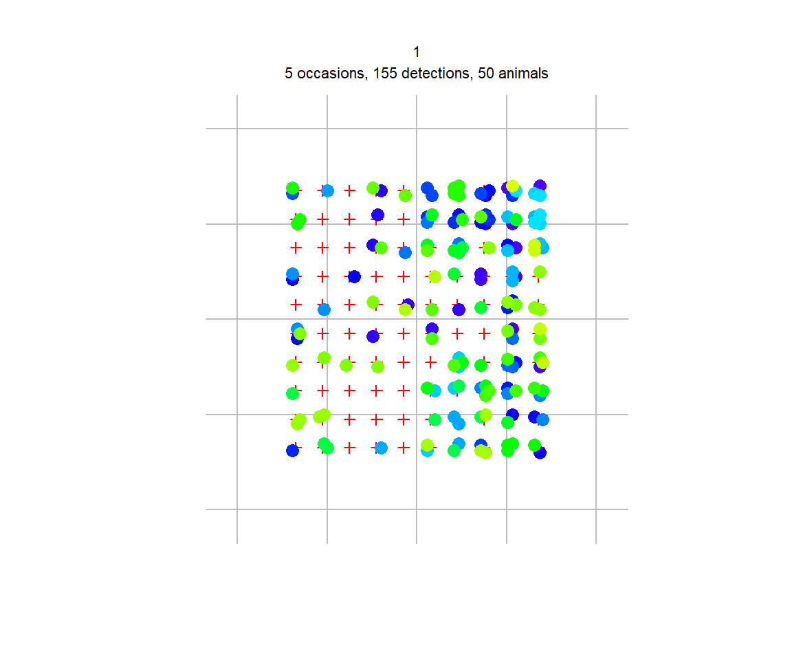

Figure I.1: Test data.

Now define a sigmoid function of covariate X:

sigmoidfn <- function (Dbeta, mask, ngroup, nsession) {
    scale <- 7.5   # arbitrary 'width' of step
    if (Dbeta[1] == "name") return ("sig")
    if (Dbeta[1] == "parameters") return (c("D1", "threshold", "D2"))
    X2 <- (covariates(mask)$X - Dbeta[2]) / scale
    D <- Dbeta[1] + 1 / (1+exp(-X2)) * (Dbeta[3] - Dbeta[1])
    tempD <- array(D, dim = c(nrow(mask), ngroup, nsession))
    return(tempD)
}

Fit null model and sigmoid model:

fit.0 <- secr.fit(ch, mask = msk, link = list(D = "identity"), trace = FALSE)
fit.sigmoid <- secr.fit(ch, mask = msk, details = list(userDfn = sigmoidfn), 
                        start = c(2.7, 500, 5.8, -1.2117, 3.4260), 
                        link = list(D = "identity"), trace = FALSE)
coef(fit.0)

         beta  SE.beta     lcl      ucl
D      3.6137 0.524474  2.5857  4.64164
g0    -1.0875 0.161739 -1.4045 -0.77051
sigma  3.3953 0.055649  3.2863  3.50439

coef(fit.sigmoid)

                beta   SE.beta       lcl       ucl
D.D1          1.6839  0.513850   0.67678   2.69104
D.threshold 514.2646 16.652893 481.62551 546.90365
D.D2          5.8810  1.047466   3.82802   7.93401
g0           -1.0860  0.161699  -1.40297  -0.76912
sigma         3.3931  0.055487   3.28439   3.50190

AIC(fit.0, fit.sigmoid)[,-c(2,5,6)]

                               model npar  logLik   dAIC AICwt
fit.sigmoid D~userD.sig g0~1 sigma~1    5 -520.64  0.000     1
fit.0               D~1 g0~1 sigma~1    3 -528.11 10.941     0

The sigmoid model has improved fit, but there is a lot of uncertainty in the two density levels. The average of the fitted levels D1 and D2 (3.7825) is not far from the fitted homogeneous level (3.6137).

beta <- coef(fit.sigmoid)[1:3,'beta']
X2 <- (300:700 - beta[2]) / 15
D <- beta[1] + 1 / (1+exp(-X2)) * (beta[3] - beta[1])
plot (300:700, D, type = 'l', xlab = 'X', ylab = 'Density', 
      ylim = c(0,7))
abline(v = beta[2], lty = 2)
abline(h = coef(fit.0)[1,1], lty = 1, col = 'blue')
rug(unique(traps(ch)$x), col = 'red')
text(400, 2.2, 'D1')
text(620, 6.4, 'D2')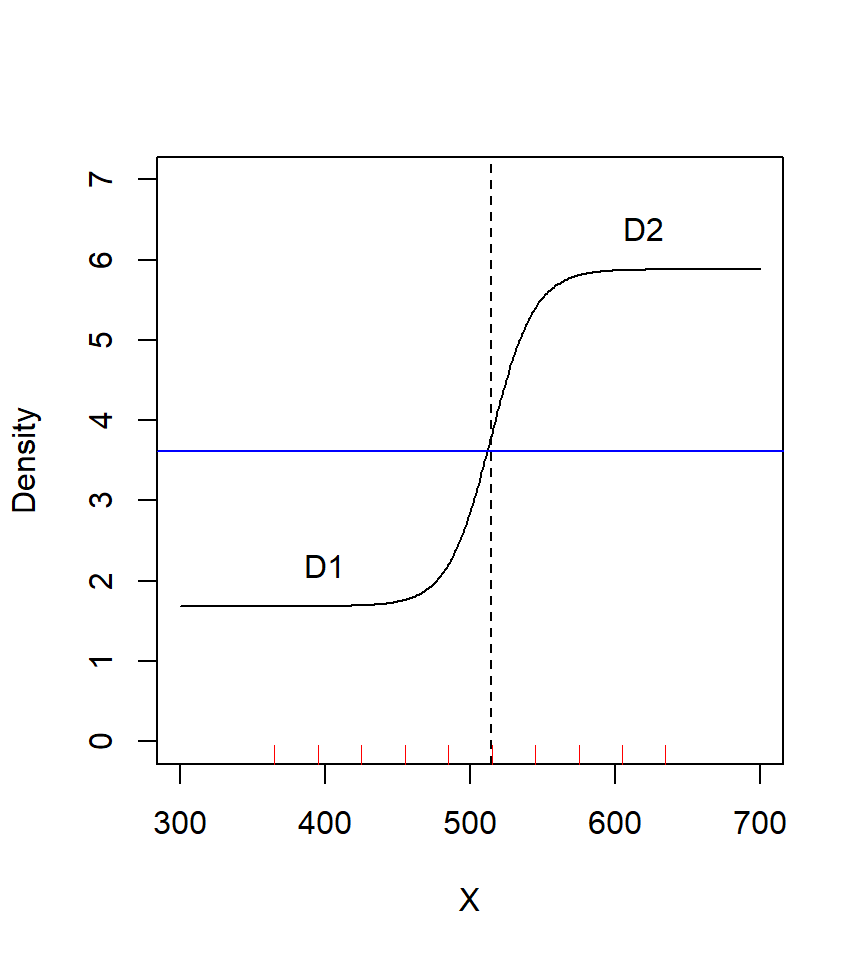

Figure I.2: Sigmoid function fitted to test data.

I.3 More on link functions

The density model for V covariates with an identity link is defined as

D(\mathbf x | \phi) = \mathrm{max} [\beta_0 + \sum_{v=1}^V \beta_v c_v(\mathbf x), 0].

From secr 4.5.0 there is a scaled identity link ‘i1000’ that multiplies each real parameter value by 1000. Then secr.fit(..., link = list(D = 'i1000')) is a fast alternative to specifying typsize for low absolute density.

Going further, you can even define your own ad hoc link function. To do this, provide the following functions in your workspace (your name ‘xxx’ combined with standard prefixes) and use your name to specify the link:

Name	Purpose	Example
xxx	transform to link scale	i100 <- function(x) x * 100
invxxx	transform from link scale	invi100 <- function(x) x / 100
se.invxxx	transform SE from link scale	se.invi100 <- function (beta, sebeta) sebeta / 100
se.xxx	transform SE to link scale	se.i100 <- function (real, sereal) sereal * 100

Following this example, you would call secr.fit(..., link = list(D = 'i100')). To see the internal transformations for the standard link functions, type secr:::transform, secr:::untransform, secr:::se.untransform or secr:::se.transform.

Kendeigh, S. C. (1944). Measurement of bird populations. Ecological Monographs, 14, 67–106. https://doi.org/10.2307/1961632