2  Simple example

In this chapter we use the R package secr to fit an SECR model to the Alaskan snowshoe hare data of Burnham and Cushwa (Otis et al., 1978).

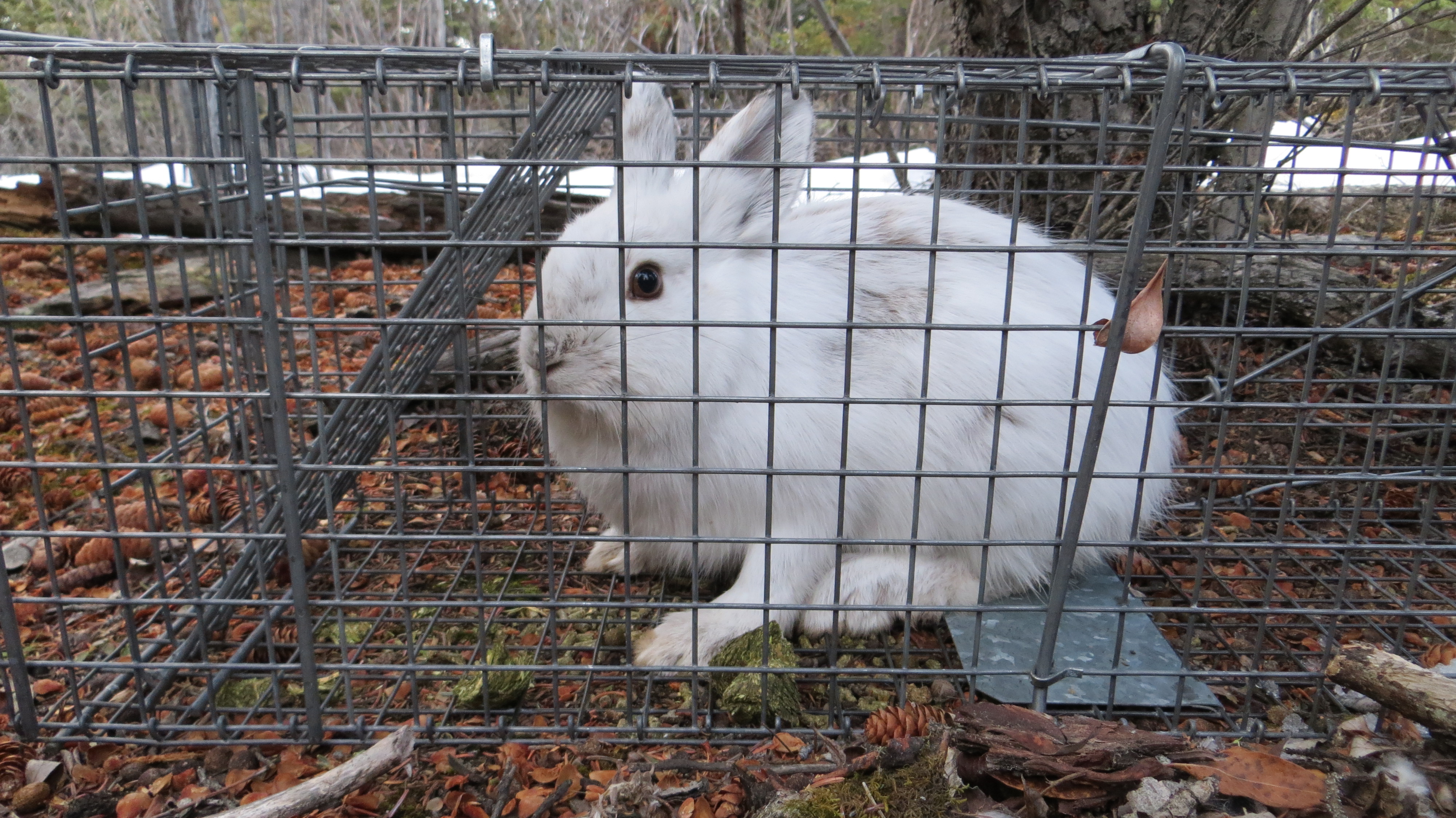
Photo: Alice Kenney

“In 1972, Burnham and Cushwa (pers. comm.) laid out a livetrapping grid in a black spruce forest 30 miles (48.3 km) north of Fairbanks, Alaska. The basic grid was 10 x 10, with traps spaced 200 feet (61 m) apart. Trapping for snowshoe hares was carried out for 9 consecutive days in early winter. Traps were not baited for the first 3 days, and therefore we have chosen to analyze the data from the last 6 days of trapping.”

Otis et al. (1978, p. 36)

2.1 Input data

The raw data are in two text files, the capture file and the trap layout file. Data from Otis et al. (1978) have been transformed for secr (code in secr-tutorial.pdf).

fnames <- c("hareCH6capt.txt", "hareCH6trap.txt")
url <- paste0('https://www.otago.ac.nz/density/examples/', fnames)
download.file(url, fnames, method = "libcurl")

The capture file “hareCH6capt.txt” has one line per capture and four columns (header lines are commented out and are not needed). Here we display the first 6 lines. The first column is a session label derived from the original study name; here there is only one session. The second column is an identifier unique to an individual (e.g., tag number). Sampling occasions are numbered 1, 2 etc. (in some studies there is only one).

# Burnham and Cushwa snowshoe hare captures
# Session ID Occasion Detector 
wickershamunburne  1 2 0201
wickershamunburne 19 1 0501
wickershamunburne 72 5 0601
wickershamunburne 73 6 0601
... 

The trap layout file “hareCH6trap.txt” has one row per trap and columns for the detector label and x- and y-coordinates. We display the first 6 lines. The detector label is used to link captures to trap sites. Coordinates can relate to any rectangular coordinate system; secr will assume distances are in metres. These coordinates simply describe a 10 \times 10 square grid with spacing 61 m.

Tip

Do not use unprojected geographic coordinates (latitude and longitude). Section C.2.1 shows how to transform geographic coordinates to rectangular coordinates (e.g., UTM).

# Burnham and Cushwa snowshoe hare trap layout
# Detector  x  y 
0101 0 0
0201 60.96 0
0301 121.92 0
0401 182.88 0
... 

After opening R, we load secr and read the data files to construct a capthist object. The detectors are single-catch traps (maximum of one capture per animal per occasion and one capture per trap per occasion).

library(secr)
hareCH6 <- read.capthist("hareCH6capt.txt", "hareCH6trap.txt", detector = "single")

No errors found :-)

The capthist object hareCH6 now contains almost all the information needed to fit a model.

2.2 Check data

First review a summary of the data. See ?summary.capthist for definitions of the summary statistics n, u, f etc.

summary(hareCH6)

Object class       capthist 
Detector type      single 
Detector number    100 
Average spacing    60.96 m 
x-range            0 548.64 m 
y-range            0 548.64 m 

Counts by occasion 
                    1   2   3   4   5   6 Total
n                  16  28  20  26  23  32   145
u                  16  24   9   9   6   4    68
f                  25  22  13   5   1   2    68
M(t+1)             16  40  49  58  64  68    68
losses              0   0   0   0   0   0     0
detections         16  28  20  26  23  32   145
detectors visited  16  28  20  26  23  32   145
detectors used    100 100 100 100 100 100   600

These are spatial data so we learn a lot by mapping them. The plot method for capthist objects has some handy arguments; set tracks = TRUE to join consecutive captures of each individual.

par(mar = c(1,1,3,1))  # reduce margins
plot (hareCH6, tracks = TRUE)

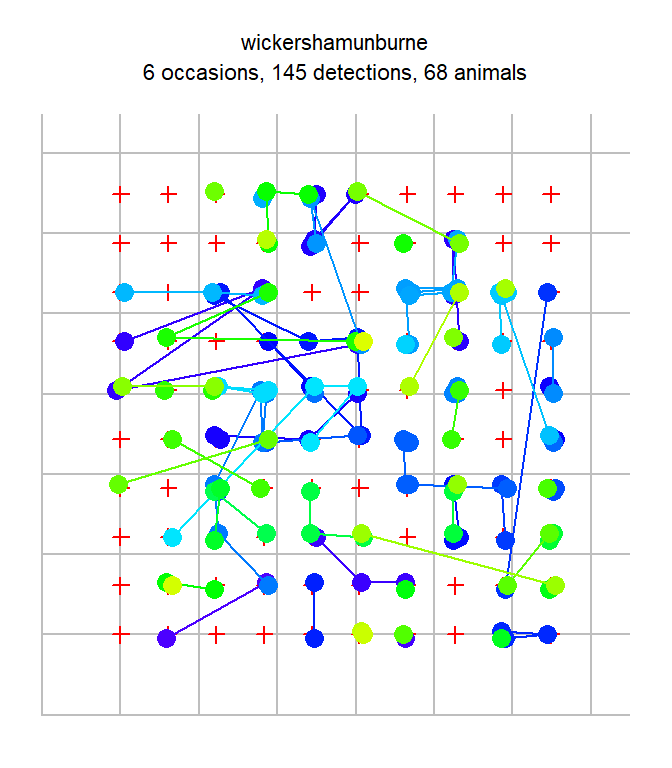
Figure 2.1: Snowshoe hare spatial capture data. Trap sites (red crosses) are 61 m apart. Grid lines (grey) are 100 m apart (use arguments gridlines and gridspace to suppress the grid or vary its spacing). Colours help distinguish individuals, but some are recycled.

The most important insight is that individuals tend to be recaptured near their site of first capture. This is expected when the individuals of a species occupy home ranges. In SECR models the tendency for detections to be localised is reflected in the spatial scale parameter \sigma. Good estimation of \sigma and density D requires spatial recaptures (i.e. captures at sites other than the site of first capture).

Successive trap-revealed movements can be extracted with the moves function and summarised with hist:

m <- unlist(moves(hareCH6))
par(mar = c(3.2,4,2,1), mgp = c(2.1,0.6,0))  # reduce margins
hist(m, breaks = seq(0,500,61), xlab = "Movement  m", main = "")

Figure 2.2: Trap-revealed movements of snowshoe hares

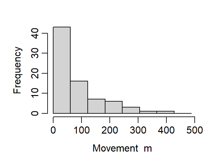
About 30% of trap-revealed movements were of >100 m (Fig. 2.2; try also plot(ecdf(m))), so we can be sure that peripheral hares stood a good chance of being trapped even if their home ranges were centred well outside the area plotted in Fig. 2.1.

2.3 Fit a simple model

Next we fit the simplest possible SECR model with function secr.fit. The buffer argument determines the habitat extent - we take a stab at this and check it later. Setting trace = FALSE suppresses printing of intermediate likelihood evaluations; it doesn’t hurt to leave it out. We save the fitted model with the name ‘fit’. Fitting is much faster if we use parallel processing in multiple threads - the number will depend on your machine, but ncores = 7 is OK in Windows with a quad-core processor.

fit <- secr.fit (hareCH6, buffer = 250, trace = FALSE, ncores = 7)

Warning: multi-catch likelihood used for single-catch traps

A warning is generated. The data are from single-catch traps, but there is no usable theory for likelihood-based estimation from single-catch traps. This is not the obstacle it might seem, because simulations seem to show that the alternative likelihood for multi-catch traps may be used without biasing the density estimates (Efford et al., 2009). It is safe to ignore the warning for now. The issue arises later as a breach of the independence assumption.

2.4 Output

The output from secr.fit is an R object of class ‘secr’. If you investigate the structure of fit with str(fit) it will seem to be a mess: it is a list with more than 25 components, none of which contains the final estimates you are looking for.

To examine model output or extract particular results you should use one of the functions defined for the purpose. Technically, these are S3 methods for the class ‘secr’. The key methods are print, plot, AIC, coef, vcov, and predict. Append ‘.secr’ when seeking help e.g. ?print.secr.

Typing the name of the fitted model at the R prompt invokes the print method for secr objects and displays a more useful report.

fit

secr.fit(capthist = hareCH6, buffer = 250, trace = FALSE, ncores = 7)
secr 5.2.1, 17:45:21 04 Feb 2025

Detector type      single 
Detector number    100 
Average spacing    60.96 m 
x-range            0 548.64 m 
y-range            0 548.64 m 

N animals       :  68  
N detections    :  145 
N occasions     :  6 
Mask area       :  104.595 ha 

Model           :  D~1 g0~1 sigma~1 
Fixed (real)    :  none 
Detection fn    :  halfnormal
Distribution    :  poisson 
N parameters    :  3 
Log likelihood  :  -607.988 
AIC             :  1221.98 
AICc            :  1222.35 

Beta parameters (coefficients) 
           beta   SE.beta       lcl       ucl
D      0.382529 0.1299502  0.127831  0.637227
g0    -2.723792 0.1609315 -3.039212 -2.408372
sigma  4.224580 0.0653229  4.096549  4.352610

Variance-covariance matrix of beta parameters 
                D          g0       sigma
D      0.01688706 -0.00173067 -0.00162336
g0    -0.00173067  0.02589895 -0.00737559
sigma -0.00162336 -0.00737559  0.00426708

Fitted (real) parameters evaluated at base levels of covariates 
       link   estimate SE.estimate        lcl        ucl
D       log  1.4659871  0.19131247  1.1363609  1.8912284
g0    logit  0.0615839  0.00930045  0.0456855  0.0825365
sigma   log 68.3457775  4.46931251 60.1324252 77.6809731

The report comprises these sections that you should locate in the preceding output:

• function call and time stamp
• summary of the data
• description of the model, including the maximized log likelihood, Akaike’s Information Criterion AIC
• estimates of model coefficients (‘beta’ parameters)
• estimates of variance-covariance matrix of the coefficients
• estimates of the ‘real’ parameters

The last three items are generated by the coef, vcov and predict methods respectively. The final table of estimates is the most interesting, but it is derived from the other two. For our simple model there is one beta parameter for each real parameter¹. The estimated density is 1.47 hares per hectare, 95% confidence interval 1.14–1.89 hares per hectare².

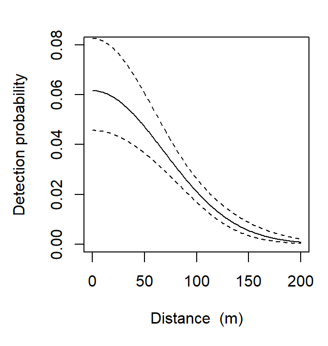
The other two real parameters jointly determine the detection function that you can easily plot with 95% confidence limits:

par(mar = c(5,4.5,2,1))  # adjust white margins
plot(fit, limits = TRUE)

Figure 2.3: Fitted halfnormal detection function, with 95% confidence limits

2.5 Revisiting buffer width

Choosing a buffer width is a common stumbling block. We used buffer = 250 without any explanation. Here it is. As far as we know, the snowshoe hare traps were surrounded by suitable habitat. We limit our attention to the area immediately around the traps by specifying a habitat buffer. The buffer argument is a short-cut for defining the potential habitat (area of integration); the alternative is to provide a habitat mask in the mask argument of secr.fit. Buffers and habitat masks are covered at length in Chapter 12.

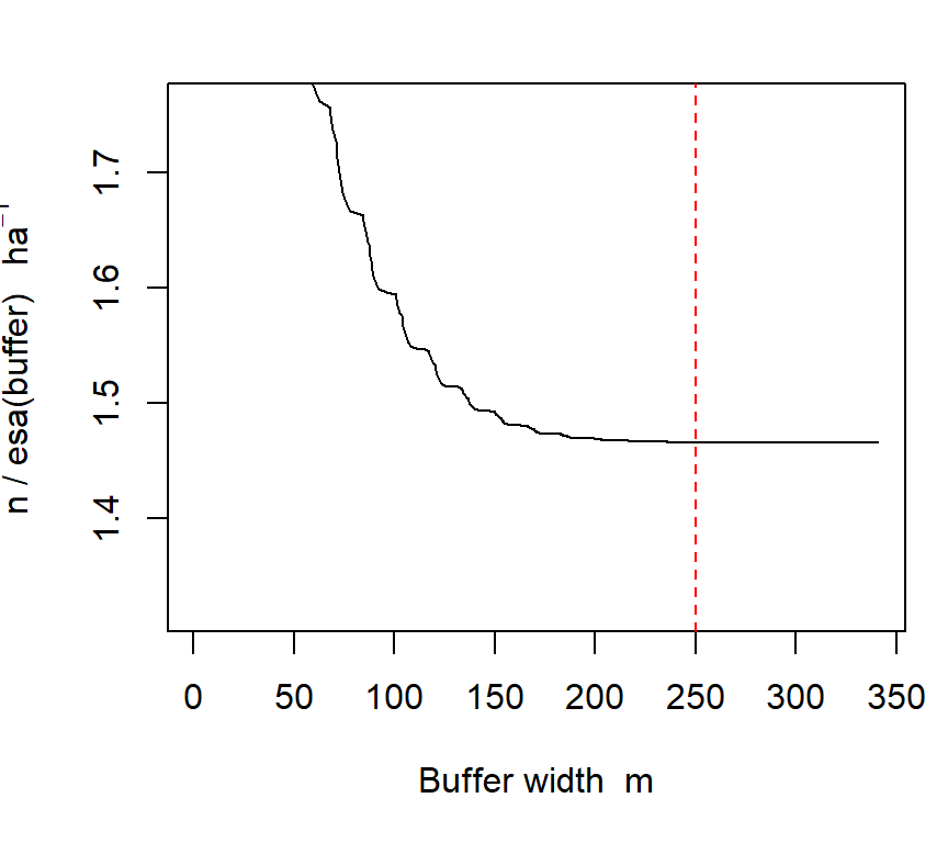
Buffer width is not critical as long as it is wide enough that animals at the edge have effectively zero chance of appearing in our sample, so that increasing the buffer has negligible effect on estimates. For half-normal detection (the default) a buffer of 4\sigma is usually enough³. We check the present model with the function esaPlot. The estimated density⁴ has easily reached a plateau at the chosen buffer width (dashed red line):

par(mar = c(5,4,2,1))  # adjust white margins
esaPlot(fit)
abline(v = 250, lty = 2, col = 'red')

Figure 2.4: Post hoc evaluation of buffer width using esaPlot()

2.6 Overall probability of detection

As a final flourish, in Fig. 2.5 we plot contours of the overall probability of detection p_\cdot(\mathbf x; \theta) as a function of AC location \mathbf x, given the fitted model. The white line is the outer edge of the automatic mask generated by secr.fit with a 250-m buffer.

tr <- traps(hareCH6)   # just the traps
dp <- detectpar(fit)   # extract detection parameters from simple model
mask300 <- make.mask(tr, nx = 128, buffer = 300)  
covariates(mask300)$pd <- pdot(mask300, tr, detectpar = dp, 
     noccasions = 6)
par(mar = c(1,1,1,5))  # adjust white margin
plot(mask300, cov = 'pd', dots = FALSE, border = 1, inset = 0.1, 
     title = 'p.(x)')
plot(tr, add = TRUE)   # over plot trap locations
pdotContour(tr, nx = 128, detectfn = 'HN', detectpar = dp, 
     noccasions = 6, add = TRUE)
plotMaskEdge(make.mask(tr, 250, type = 'trapbuffer'), add = TRUE, 
     col = 'white')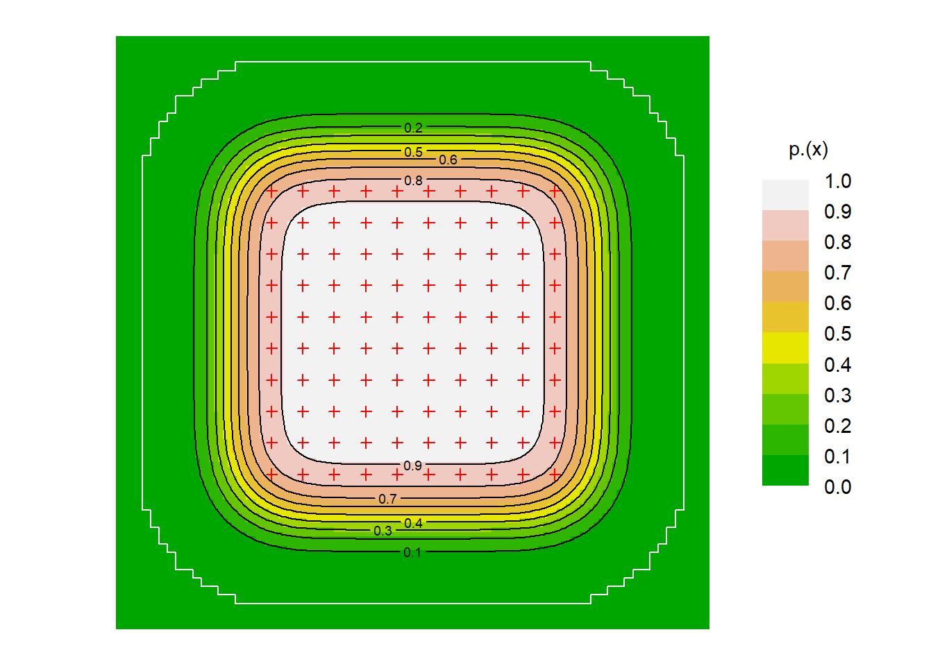

Figure 2.5: Contour plot of overall detection probability p_\cdot(\mathbf x; \theta).

covariates(mask300)$pd <- pdot(mask300, tr, detectpar = dp, 
    noccasions = 6)
covariates(mask300)$d <- distancetotrap(mask300, tr)
covariates(mask300)$dclass <- cut(distancetotrap(mask300, tr),
    c(0,100,200,400))
par(mar = c(4,4,2,2))
f <- c(0,0.1,0.2,0.3,0.4,0.5)
nm <- nrow(mask300)
hist(covariates(mask300)$pd, xlim = c(0,1), ylim = c(0,nm/2), 
     breaks = seq(0,1,0.05), col = 'forestgreen', axes=F,
     ylab = "Fraction of mask population",
     xlab = "Overall probability of detection", main = "")
axis(1)
axis(2, at = nm * f, labels = f)
for (i in 0:9)
hist(covariates(mask300)$pd[covariates(mask300)$pd>i/10], breaks =
      seq(0,1,0.05), add = T, col = terrain.colors(10)[i+1])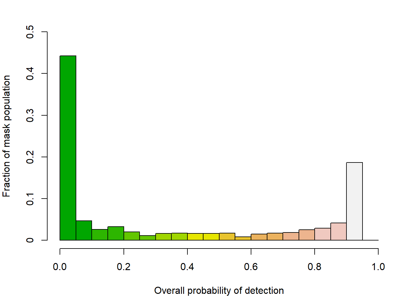

Figure 2.6: Distribution of overall detection probability p_\cdot(\mathbf x; \theta) for AC within the area of Fig. 2.5.

Efford, M. G., Borchers, D. L., & Byrom, A. E. (2009). Density estimation by spatially explicit capture-recapture: Likelihood-based methods. In D. L. Thomson, E. G. Cooch, & M. J. Conroy (Eds.), Modeling demographic processes in marked populations (pp. 255–269). Springer.

Kendeigh, S. C. (1944). Measurement of bird populations. Ecological Monographs, 14, 67–106. https://doi.org/10.2307/1961632

Otis, D. L., Burnham, K. P., White, G. C., & Anderson, D. R. (1978). Statistical inference from capture data on closed animal populations. Wildlife Monographs, 62.

---

1. We can get from beta parameter estimates to real parameter estimates by applying the inverse of the link function e.g. \hat D = \exp(\hat \beta_D), and similarly for confidence limits; standard errors require a delta-method approximation (Lebreton et al. 1992).

2. One hectare (ha) is 10000 m² or 0.01 km².

3. This is not just the tail probability of a normal deviate; think about how the probability of an individual being detected at least once changes with (i) the duration of sampling (ii) the density of detector array.

4. These are Horvitz-Thompson-like estimates of density obtained by dividing the observed number of individuals n by effective sampling areas (Borchers and Efford 2008) computed as the cumulative sum over mask cells ordered by distance from the traps. The algorithm treats the detection parameters as known and fixed.